MICROGRAD FOR MORTALS

TL;DR Let’s use Micrograd to explain core ML concepts like supervised learning, regression, classification, loss functions, and gradient descent. We’ll break down how models adjust weights and biases during training using backpropagation. Through simple code examples, it visualizing how gradients flow through a minimalistic neural network.

Intro 

This article deviates from the usual offensive tradecraft and dives instead into the world of Machine Learning (ML). For this first post, I’ll lean into Micrograd and its simple yet clever approach. The intent here is to leverage this project and observe some of the most basic ML concepts in action. I’m not an ML engineer; I just found Micrograd to be a great tool for explaining fundamental ML ideas and I would like to share that with anyone who finds themselves at the start of their ML learning journey.

I’d like to start by pointing out that the creator of Micrograd and one of the top ML talents in the world, Andrej Karpathy has a video walkthrough on his project, in which he not only explains and demonstrates the inner workings of the code but also gives insight into some of the design choices behind it. I recommend watching it as well.

Content

Right after a quick intro to Microgard, this post can be divided into two major sections.

The first is an ML crash course, so terms like back-propagation, gradient descent, and others don’t catch us off guard. Rather than just listing definitions for each of the related terms and concepts, I thought it would be more valuable to step through them with examples and come out on the other side with a solid knowledge base and ready to explore Micrograd.

In the second portion of this article, we’ll take advantage of Micrograd and its minimalistic approach to expand on the concepts from the first section while we step through a barebones basic round of model training.

The end goal of this post is to understand core concepts about how a model learns to perform tasks like generating poetry sonnets, properly classifying pictures of cats vs dogs, or even making a prediction about next week’s rainfall based on a single prompt.

Intro

What is Micrograd (and What Does it Do)?

Micrograd is a minimalistic automatic gradient engine implemented in Python, capable of performing core ML steps, such as backpropagation and others. More importantly for the purpose of this post, the project makes it possible for us to visualize and track these steps. 

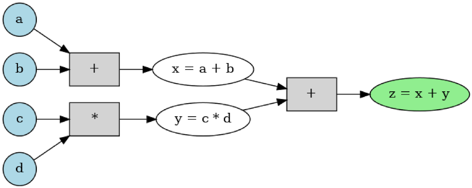
The code gives us the ability to work with atomic components, like scalars (single values), making it easier to follow along the backpropagation process with a Directed Acyclic Graph (DAG). A DAG will help us track a chain of operations and its components from beginning to end.

Another big plus for using the project is that in its current state, the code consists of 154 lines of simple yet pretty clever Python code, adding another point to the “Great for Learning” category.

Before jumping into Micrograd’s inner workings and to better understand the steps we’ll take in that section, let’s cover some basic Machine Learning concepts.

0-60 Machine Learning Crash Course

What is ML?

ML is the process of training a model, which in its simplest form is just a piece of software. We train a model to be able to generate predictions or content based on the data that is fed to it as input. The goal is to have this software’s output be as accurate and valuable as possible.

Model Training Paradigms

There are different approaches when it comes to training a model. Choosing the most suitable one will generally depend on the type of prediction or content that we want as output of our model. This means that if we want our model to recognize and classify pictures of cats vs dogs, we’ll use slightly different training techniques than if we want it to be able to write Shakespeare-sounding paragraphs.

Supervised Learning

For this approach, we feed the model a controlled set of data and, in parallel, we also provide it with the corresponding correct predictions based on that data. This is done to let the model learn the relationship between the data provided as input, also known as features, and what is known to be the right answer or output, sometimes referred to as labels or targets.

Think of it as seeing different playbooks that a basketball team has and then getting to see the final score for the games where each of those playbooks was used. After reviewing some of them we would probably get a good idea of the relationship between some of the provided playbooks (input as features) and how well the team performed at that particular game (resulting labels). Taking it a step further, you could learn the plays that have more influence on a winning score and change the playbook to increase the relevancy of such plays to increase the chances of winning future games.

Depending on the goal of the model, there are a lot more layers to Supervised Learning, which can help train it to be as accurate and efficient as possible. We’ll cover some of that in the Model Training and Goals section.

Unsupervised Learning

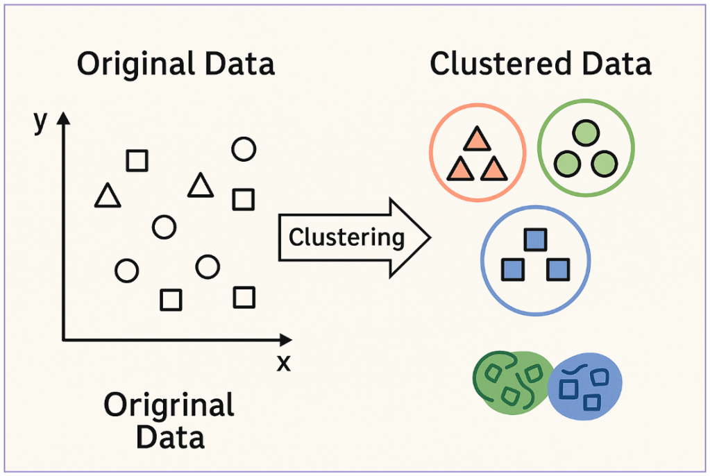
Another approach to model training is to provide input data to it, but then let the model come up with its own conclusions. This can be referred to as Unsupervised Learning. Here we look for the model to find relationships amongst provided input data groups. A model trained with this approach will commonly employ a technique called clustering. Here the model will demarcate “natural” groupings (clusters of data) based on what it sees in the data.

An unsupervised approach can be useful in situations where we want to analyze data and find relationships and patterns that we were not previously aware of or that would be very resource demanding to figure out with just manpower. For example, a model could analyze user behavior within an Active Directory environment. We could then train our model to learn prevalent login patterns and make it easier to identify abnormal behavior for that particular account.

The model training approaches we just covered are not exclusive and can be aggregated to work on top of or alongside each other, which is what we’ll see in most real-world LLMs. 

These types of training can also be layered with fine-tuning techniques like reinforcement learning where correct or accurate predictions are rewarded and incorrect ones are punished (Some resources will consider reinforcement training to be its own category of training paradigm).

Model Training and Goals

We previously mentioned that choosing a training paradigm would depend on what we are looking for as the output of our model. Let’s look at some common types of goals for ML models and pick a couple to dig into:

• Regression
• Classification
• Clustering
• Generative Modeling
• Anomaly Prediction

There are even more approaches than those listed for training a model and the limit here is just based on human creativity. 

To maximize our learning journey we’ll continue to focus on Regression and Classification.

Regression Models

We will often see models that output a single value as their only task. For example, a model that predicts the chance of rain for a certain day of the week in a certain area, or hear me out…  predict 0 to 60 acceleration times based on engine horsepower and other characteristics of an automobile.

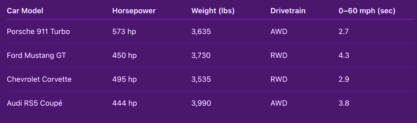
This type of model is known as a regression model. A regression model looks to learn the relationship between the data that we provide to it (e.g., horsepower, weight, drivetrain) and a certain result or output (e.g., 0-60 mph/sec). A model can learn this by employing a supervised training approach, where we provide the data to it as well as corresponding correct answers (labels). With that, we can train it to be able to make predictions that are as close as possible to those labels. We will cover more on this in the Loss section of this post.

Classification Models

The canonical example for a classification model is an email spam filter and we’ll continue with that tradition here. 

A model could be trained to classify emails as being spam or not based on characteristics like certain words being part of the message body, the domain associated with the sender, and more. Some other use cases for a classification model can be classifying network traffic or software as malware-related or benign.

A classification model can also employ a supervised learning approach with the goal to find the relationship between the characteristics of the input data, for example a dylib library, and what is  known to be a malicious action on a host, say accessing TCC protected locations on a macOS host.

Now that we have a better idea of how those two approaches differ from each other, let’s go a little deeper into the model training process.

What Happens During Model Training:

When taking a supervised training approach, the input data we provide will be known as our dataset. This is the entire set of information that we want to use to train our model in its early stages.

During training, the model will follow repetitive cycles to run this data through a statistical technique like linear regression for a regression model or logistic regression for a classification model. This means the model will run the data through a mathematical function like the following one for linear regression:

In this case:

• y =  the model’s resulting output
• x =  provided input or data 
• b =  the model’s bias
• w = the weight associated with features

We’ve talked about data and output, but here we see a couple of new components. Let’s clarify the role of Bias and Weights in model training.

Bias

If we were to see a linear regression function as a graph, the Bias would be the starting point of the model on the y-axis.

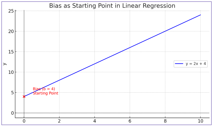
This can be thought of as what the model thinks should be included in the prediction, regardless of any intricacies and characteristics of the input data we provide. Working through an example, let’s say we are trying to calculate the fuel cost for different road trips we make throughout the year. Let’s also say that, regardless of how far we go, we always want to let the engine warm up for five minutes before we leave our driveway. In that case, our calculations would always start with the value of the cost of warming up the engine before starting the trip.

We’ll assume our warm-up routine costs $0.25 ( insert here all those “Five reasons why warming up your car is super very bad” … but also “Five reasons why warming up your car is the best maintenance hack”) and, with that, our logistic regression function should start taking shape:

In this example, x (i.e., the provided data) will be the distance of each trip. Regardless of that, our prediction will always start with the fact that we will spend $0.25 every trip, which would be the Bias in our calculation.

Weight

Let’s continue with the previous example and say that when gathering information for our fuel cost trip estimation, we get a bit carried away and end up throwing in a lot of different information into the mix. Some of that information can be very useful for our estimations (e.g., the trip happens during peak or off-peak hours) and some not so useful, like the type of music we listen to during the trip. Some might disagree on the importance of that second piece of data which is totally fair!

After some training rounds, the model might learn that maybe the radio station does not have as much influence on the fuel cost of our trip compared to the time of the day (again, fair to disagree on this one). So, as part of its training, the model will adjust itself to give some more Weight to one of those, and this is done to have its predictions be more accurate.

So, Bias and Weight are parameters of our model that will influence the output. The model will self-adjust these parameters as part of the training process while it learns which parameters should matter the most for what it is asked to do or predict. In early training stages, most often these parameters start with a random number.

Putting our examples together, now we know that our linear regression function could be seen as:

Since this is a linear regression function, this would be applicable for a regression model. Let’s continue looking at what actually happens during model training, this time within classification models.

Classification Cases

In the previous example, we saw a model that outputs a single value (i.e., calculated fuel cost of a trip), which would be in line with a regression model. In the case of a classification model, the difference will be that we need the model to translate a resulting value into the probability of the data belonging to a certain class. 

Let’s go back to that email spam case. If our model runs that same example data through a function and ends up with a value of 9.765, that value by itself (single output) would not be much help in determining if an email is spam or not or classifying a road trip cost as expensive vs economical.

To achieve that desired categorization, classification models will rely on a logistic regression function instead of a linear one. This will allow the model to transform the resulting value into an unsigned number that represents the probability of affiliation. Combining that with the concept of classification thresholds will allow a model to learn and separate a benign email from a spam one, depending on where they land in relation to such a threshold.

A logistic regression function is not too far from a linear regression one like the one we saw in the previous section. In its simplest form, this type of function would be:

• x  = input data
• y = resulting prediction
• o = Sigmoid function
• b = bias
• w = weight

For this simple log reg example, the most notable difference will be the Sigmoid. Lets see what role it plays in training a classification model.

Sigmoid

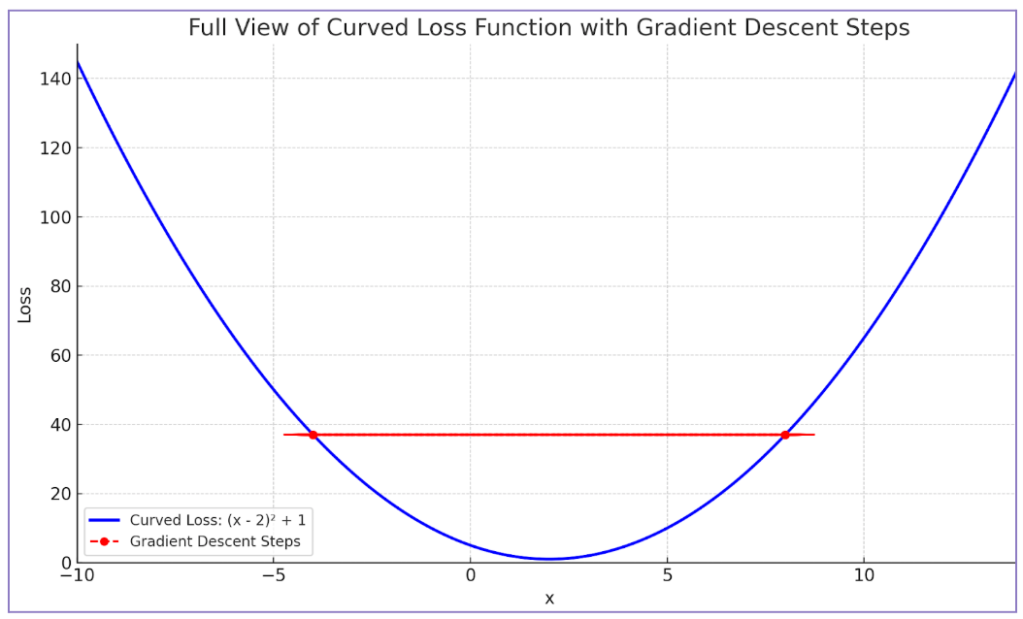
A sigmoid function is a logistic function that transforms a value into a representation that lives between 0 and 1. During training, the model will leverage a sigmoid to squish a resulting value to fit within that range. If we were to represent the relationship between input data and predictions in a graph, a sigmoid will turn a linear vector into a curved or S (hence Sigmoid) shaped vector.

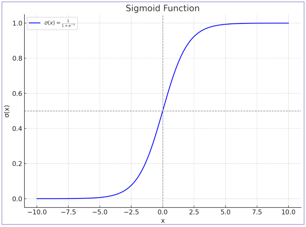
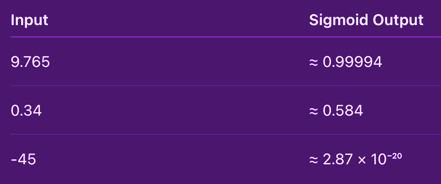
We’ll continue with our beloved spam example to try and make this concept easier. Let’s say that we have an email spam classification model with predictions resulting in the values 9.765, 0.34, -45. With a large model, keeping track of such a wide range of values in regard to the probability of being spam or not could be very resource-consuming. As an alternative, a logistic regression will run each of those values through a Sigmoid and end up with a corresponding value between 0 and 1.

If we pass our example prediction values (9.765, 0.34, -45) through such a function and then set our model to have a spam threshold of 0.5, where anything above that will be considered spam and anything below will go to the inbox, we would observe that starting from top to bottom, the first email was very likely spam; the second was barely spam; and the third one was absolutely not spam according to our model predictions.

In ML, a classification model will have an established threshold and any resulting values between 0 and 1 will be mapped against that threshold.

As usual, there are layers to this. There are a multitude of different Sigmoid functions with different resulting value ranges and characteristics and the same applies to thresholds. By comparison in the real world, we’ll see that it is usually not so black and white as setting the value at 50%. Factors like the implications of sending an email that is not spam to the spam folder can help us determine a more useful denominator. For example, most spam filters want to be more certain than 50% in order to send something to the spam folder.

Now that we have a better idea of what takes part in the process of training a model to make predictions and the role that linear and logistic regression play in that, let’s see how the model determines when its predictions are correct; when they are wrong; and how it actually learns to make those predictions/classifications as accurate as possible.

Loss

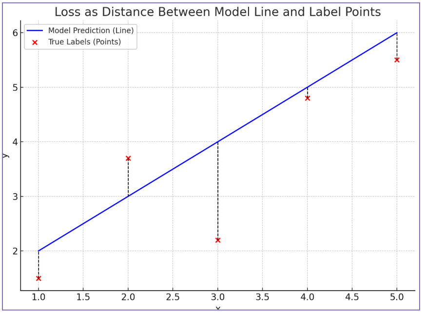
Loss in ML refers to the quantitative difference between the model predictions and the labels. Simpler; loss lets a model know how far its predictions are from the correct answers

In a graph, Loss can be viewed as the distance between the line that represents the model, or its predictions, and the markers that represent the Labels, or values known to be the correct answers.

Sounds simple enough, right? There are, however, different layers and approaches to calculating Loss; most with the goal of optimization. Some of those approaches are:

• L1 Loss / Mean Absolute Error
• L2 Loss / Mean Squared Error
• Log Loss

I won’t dive too deep into each of those, but these consist of formulas meant to end up with a single Loss number. Some will calculate the sum of all losses resulting from a data example and some work with their average instead. In all those cases, the Loss will be a positive number. That is because these functions either just get the absolute value of the Loss or they square up the result to get rid of negative signs. 

The following resource does a good job at covering the most common ones; Five Essential Loss Function Techniques for ML Success.

The goal of training our model in ML is to reduce the Loss to the lowest possible value, because this means that the difference between our model and the known correct answers is at its minimum. Achieving this is known as convergence.

Achieving Convergence

Let’s see how a model can reduce Loss as part of its learning by adjusting its parameters (i.e., Bias and Weight).

Once a model makes an initial round of predictions based on input data, and then measures  how wrong or right those were (Loss), the model will go back through all the different operations that generated the Loss and start calculating how much each operational component (i.e., Nodes) influenced the resulting Loss value. For example, here we have a series of operations which lead to a result represented by d:

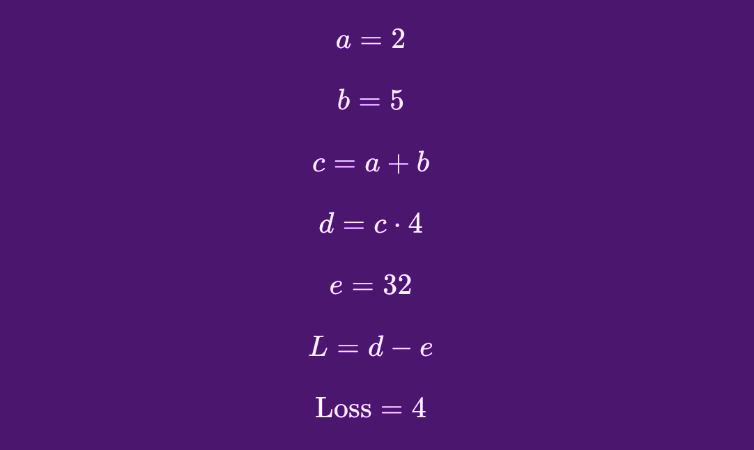
In this particular example, the label was provided as e = 32. Calculating Loss (d minus e) here leaves us with Loss = 4. With that information the model will try to go backwards through the chain of mathematical operations and determine how much each of the components had a say in the final value being 4. This gradient calculation process is a basic component of Backpropagation.

Backpropagation

Backpropagation is the process that a neural network model goes through to determine the amount of influence certain components had on a final result.

Let us adjust this concept to better fit our example. Backpropagation is the process of finding the derivative of the result in relation to each of the nodes that made part of the chain of operations that resulted in Loss = 4. 

Like finding the derivative of Loss = 4 in relation to b = 5. In other words, how much influence b had in the Loss being 4

Continuing with this example, there are different derivative rules for the different types of operations but essentially we would break up a chain of operations that gave us our resulting value and then find the derivatives for each node part of those operations. 

So for this:

We would find the derivative of L with relation to a or dL/da and dL/db, dL/de, and so on until we have completely mapped the chain of operations that led to our final result and their corresponding derivatives.

Until now, in order to keep it simple, we’ve been only talking about derivatives which generally refers to functions with a single input. To better understand Loss and backpropagation, it is best to start making the switch to gradients.

Gradients

Are a more appropriate measure unit when working with multiple input functions. If we put them in a graph where we are showing a model based on multiple features, gradients represent the slope of that line at a particular point. 

In ML terms and simplifying a bit the gradient represents how a particular point in the model line influences the direction of that line. For example, if we are at a particular point in a linear model graph and we edit the values that point represents, the gradient tells us how much that would influence the next point in the model.

A model will use gradients during training to figure out the right direction of adjusting parameters (towards positive or negative quadrant) to reduce the Loss. If the gradient at a certain point indicates that following that course will augment the Loss then the model should look to change those values in a direction opposite to such gradient.

Once our model reaches the lowest possible amount of Loss, then it has achieved convergence. However, how fast and how easy convergence is achieved depends on different factors of our training approach; factors like hyperparameters.

Hyperparameters

These are parameters that we will configure for our model to use during training. These can be:

Batch Size

This is the number of examples that we want our model to make predictions on before updating its parameters. Most often, the entire data set will be divided into batches and batches into data examples. This is done so we can take advantage of the parallelism that a CPU allows for, meaning we can train on multiple batches simultaneously, which can lead to faster convergence.

Epoch

An epoch in ML training just means that the model has completed a pass through the entire dataset (all data examples and batches).

Learning rate

The learning rate determines the size of the adjustments done to the parameters when the model strives to reduce the Loss. 

Now that we’ve covered some of the most basic concepts of ML, let us take the knowledge gained and use Micrograd to see these concepts in practice.

Micrograd … Finally

Now we can begin to leverage Micrograd and observe the basic inner workings of ML The project’s repository readme page greets us with the following example:

Example usage

Below is a slightly contrived example showing a number of possible supported operations:

from micrograd.engine import Value

a = Value(-4.0)
b = Value(2.0)
c = a + b
d = a * b + b**3
c += c + 1
c += 1 + c + (-a)
d += d * 2 + (b + a).relu()
d += 3 * d + (b - a).relu()
e = c - d
f = e**2
g = f / 2.0
g += 10.0 / f
print(f'{g.data:.4f}') # prints 24.7041, the outcome of this forward pass
g.backward()
print(f'{a.grad:.4f}') # prints 138.8338, i.e. the numerical value of dg/da
print(f'{b.grad:.4f}') # prints 645.5773, i.e. the numerical value of dg/db

Even though it looks quite complex, and I will paraphrase the creator here, “These operations don’t mean anything, they are just there to flex about what Micrograd can do”. The example is meant to demonstrate the different types of operations that Micrograd can track. 

If we recall some of the examples from the crash course section (trip fuel cost), a model needs to understand which parameters have the most influence on its predictions to adjust them effectively and improve accuracy; parameters like weights associated with peak and off-peak trip values. To do this, the model must keep track of how a particular prediction was made and this includes the sequence of operations that led to it. This is where backpropagation comes in. 

Manual Backpropagation

Backpropagation involves computing the gradient for each node part of the chain of operations (from a forward pass) that make up a model. 

Let us observe this by stepping through a manual backpropagation example. This will also help us understand how Micrograd handles and displays data. We’ll leverage some useful Python libraries for the rest of the post.

import inspect
import math
import random
import numpy as np
import matplotlib.pyplot as plt
%matplotlib inline

We can start with a simple sequence of operations like this one.

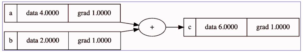
a = Value(4.0)
b = Value(2.0)
c = a + b

print(c)

Value(data=6.0, grad=0)

Working backwards through the chain of operations, we can manually perform and observe a single backpropagation step by finding out how much influence a has over the final result being 6.0.

Attempting to determine the gradient of c in relation to the following node backwards, we can see that c resulted from doing a + b, and we know that the derivative rule for a sum operation is just 1. So, in this case a.grad will be 1.

a = Value(4.0)
b = Value(2.0)
c = a + b

a.grad = 1

print(a)

Value(data=4.0, grad=1)

Since both a and b affect the result of c through a sum operation b.grad will be 1 as well. This is telling us that a influences c by a magnitude of 1. Another way to put it is that c is equally sensitive to changes in a or b, by a degree of 1.

Why Value()?

We just performed a micro backpropagation step and found the gradient we were interested in; however, at this point, you might be wondering why are we declaring values like this, a = Value(4.0), and not just a = 1 like we would usually do with Python. To answer that, let’s see how Micrograd would approach our previous manual step. 

Looking into the code of the project’s engine.py file, we’ll focus on the following class methods.

class Value:
    """ stores a single scalar value and its gradient """

    def __init__(self, data, _children=(), _op=''):
        self.data = data
        self.grad = 0
        # internal variables used for autograd graph construction
        self._backward = lambda: None
        self._prev = set(_children)
        self._op = _op # the op that produced this node, for graphviz / debugging / etc

The first can be found at the beginning of the script. The code is pretty simple. It declares a Value class and its constructor method, where it sets some attributes that an object of this class will have.

def __repr__(self):
  return f"Value(data={self.data}, grad={self.grad})"

The second method, shown above, can be found at the end of the engine.py file. This part just tells Python what to do when somebody calls print() on an object of the Value class.

In our initial example, we created the object a and gave it a value of 4.0. Then we ended up with a Value object that has its .data property set to 4.0 , and its .grad property set to 0, as well as other properties set to default values, which we can leave aside for now.

Calling print() on that object, we get:

print(a)

Value(data=4.0)

A complicated way of just printing 4.0? There must be a reason to take this approach after all.

As part of our manual step, to calculate the gradient we needed to know that c came from a + b. Micrograd also needs a way to know this when performing backpropagation. Native Python alone does not support this. So, if we were to try something like:

a = 4
b = 2
c = a + b

print(c.grad)

Asking Python to give us the gradient of c in relation to b would give us this:

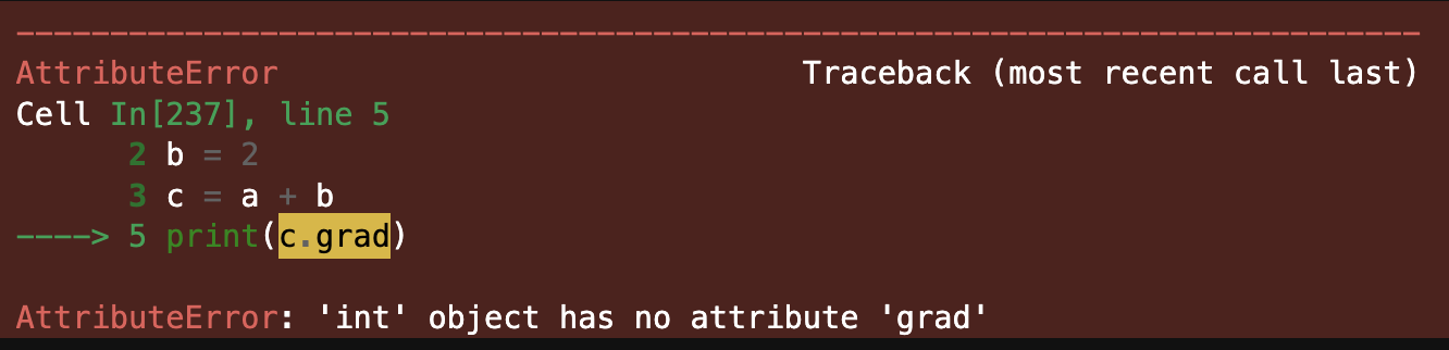
This is expected, since int objects don’t have a grad attribute. More importantly, Python does not know what came before c, which is required to calculate the derivative of c in relation to a. For that, the code needs to know the derivative rule for a sum operation.

Even for such a small chain of operations, the list of steps to track can get extensive quite  quickly.

That is where the Value class comes in handy. Having an object of this class is what allows Micrograd to add custom attributes to that very same object, attributes that can be stored and tracked. For example, attributes that can tell us what came before another and which operands were involved in its making.

Tracking a Chain of Operations With Micrograd  

If we look at the method that follows the Value class declaration, we see:

def __add__(self, other):
    other = other if isinstance(other, Value) else Value(other)
    out = Value(self.data + other.data, (self, other), '+')

def _backward():
self.grad += out.grad
other.grad += out.grad
out._backward = _backward

return out

This is a Python overload method and basically is telling Python what to do when someone tries to sum two objects of the Value class (i.e., Value(4.0) + Value(2.0)). Within this __add__ method, the code takes both of those objects and creates a new Value object. It then stores each of the original object values 4.0 and 2.0 as children of that new object. 

As a result, the self._prev attribute of the new object will be populated with a Python set containing the children of the current object. It also stores the operand used against those children nodes in the self._op attribute (i.e., +). Still within the addition operation overload method, we’ll find a nested private method called _backward, and within this function we’ll see that the code is calculating the gradient for each of the children nodes used in the __add__ operation. 

def _backward():
    self.grad += out.grad
    other.grad += out.grad

Micrograd sets the gradient of self.grad to out.grad. For this example and for this type of operation the gradients will be equivalent to each other.

The Value in a Value Class: 

Now we know that Micrograd uses this class to keep track of objects that are the result of other Value class objects and the operations between them. It leverages this to calculate and store their gradients as well as other useful attributes. 

Reviewing later parts of the code, you’ll see that it takes the same approach for other operations as well (i.e., multiplication) and it employs different derivative rules in order to find the corresponding gradients.

def __mul__(self, other):
    other = other if isinstance(other, Value) else Value(other)
    out = Value(self.data * other.data, (self, other), '*')

    def _backward():
        self.grad += other.data * out.grad
        other.grad += self.data * out.grad

    out._backward = _backward

    return out

The best part is that, thanks to this clever and minimal code, we don’t actually need to perform manual backpropagation to be able to observe manual backpropagation. Even better, we can do this with a much easier to digest Directed Acyclic Graph (DAG). The corresponding DAG lets us see each of the nodes part of a chain of operations, their current data values, the associated labels and more importantly … their gradients.

With Micrograd we can generate those gradients automatically by calling the .backward() method on the node we are interested in. Taking the c node as an example.

c.backward()
draw_dot(c)

And then generating a DAG with graphviz by calling draw_dot on it.

Growing Into Neural Networks

As we continue piecing the puzzle together and move closer to observing an actual model training scenario, it’s helpful to learn more about the model structure it supports.

One of the reasons why Micrograd makes for a good learning tool is because it can work with  (at least in the beginning) scalars, which for this post we can just think of as single value representations. 

Unfortunately, scalar values by themselves are not an accurate rendering of a neural network. A neural network is a type of model that gets inspiration from the human brain structure and its layers of connected nodes. This, along with transformers (which is a special type of neural network), is one of the foundations of most LLMs we see nowadays. 

In general, a neural network will be formed by a perceptron as its basic unit which in turn will be formed by multiple neuron layers. 

Neuron

A neuron in ML is a mathematical representation of a biological neuron. That will look something like this.

Here, we see multiple different inputs that interact against different weights and then each resulting interaction flows into the cell body of the neuron. Within the cell body of a neuron, we add a bias value and then pass the result of all that through some kind of activation function.

Activation Functions

In the context of a neuron, an activation function decides whether the neuron should pass its output to the next layer based on the input it receives.

Without the activation function, the neuron would just output a straight line. This would take away the network’s ability to learn more complex patterns. An activation function introduces non-linearity, allowing models to handle things like curves, language, or images. Some common examples of this are sigmoid, tanh and ReLU functions.

Putting these pieces together, building a neuron step-by-step could be seen as the following. 

1. The input x → interacts with a weight w. So, we have x * w, 
2. That would flow into the cell body where the bias is added to it, which would end up looking like b + (x * w). 
3. Passing that through a Sigmoid function would leave us with something that hopefully seems familiar from the 0-60 Machine Learning Lightning-Fast Crash Course – Classification section.

Putting those Neuron building steps together gave us something very similar to a logistic regression function. 

Throwing in an extra layer of real-world complexity, a typical neuron will receive multiple inputs. That function will be more along the lines of this:

Micrograd Neurons

Let’s see how these Neurons are implemented in Micrograd.

class Neuron(Module):

    def __init__(self, nin, nonlin=True):
        self.w = [Value(random.uniform(-1,1)) for _ in range(nin)]
        self.b = Value(0)
        self.nonlin = nonlin

    def __call__(self, x):
        act = sum((wi*xi for wi,xi in zip(self.w, x)), self.b)
        return act.relu() if self.nonlin else act

    def parameters(self):
        return self.w + [self.b]

    def __repr__(self):
        return f"{'ReLU' if self.nonlin else 'Linear'}Neuron({len(self.w)})"

In Micrograd, the file nn.py defines a Neuron class. The constructor of the class takes the number of inputs as nin and defines a .w as the weight attribute and .b  as the bias attribute for the object. It also defines if the function is linear or not. These neurons are to be used as input into the MLP (Multi-Layer Perceptron) constructor method which sits in the continuing lines of code. We can see a neuron for our model.

values = [4.0, 2.0]
NRN = Neuron(2, [3, 3, 1])
NRN(values)

Value(data=2.3740860347383608)

Next in the code, the layer class is defined and in turn it creates a layer of neuron objects. A layer in this case is just a set of neurons from which the model calculates a result. It does this in the same way we have been calculating predictions leveraging a linear or logistic regression function.

class Layer(Module):

    def __init__(self, nin, nout, **kwargs):
        self.neurons = [Neuron(nin, **kwargs) for _ in range(nout)]

    def __call__(self, x):
        out = [n(x) for n in self.neurons]
        return out[0] if len(out) == 1 else out

    def parameters(self):
        return [p for n in self.neurons for p in n.parameters()]

    def __repr__(self):
        return f"Layer of [{', '.join(str(n) for n in self.neurons)}]"

The constructor method for this class receives the quantity of neurons that will be part of the  layer.

MLP’s

To complete a Micrograd neural network we have the MLP class. This is Micrograd’s  Multi-Layer Perceptron implementation. We can define an object of the MLP class as having a certain number of inputs (neurons), a certain number of layers, and lastly the number of outputs (we’ll keep it as a single value for our example). 

Overall, the approach of this method is very much like the previous layers with the difference that the inputs are taken as groups rather than single objects. 

class MLP(Module):

    def __init__(self, nin, nouts):
        sz = [nin] + nouts
        self.layers = [Layer(sz[i], sz[i+1], nonlin=i!=len(nouts)-1) for i in range(len(nouts))]

    def __call__(self, x):
        for layer in self.layers:
            x = layer(x)
        return x

    def parameters(self):
        return [p for layer in self.layers for p in layer.parameters()]

    def __repr__(self):
        return f"MLP of [{', '.join(str(layer) for layer in self.layers)}]"

Let’s define an MLP that will consist of two inputs into three layers of three neurons each and have all that come out into a single output.

values = [4.0, 2.0]
MLP = MLP(2, [3, 3, 1])
neuralN(values)

Let’s go ahead and graph it.

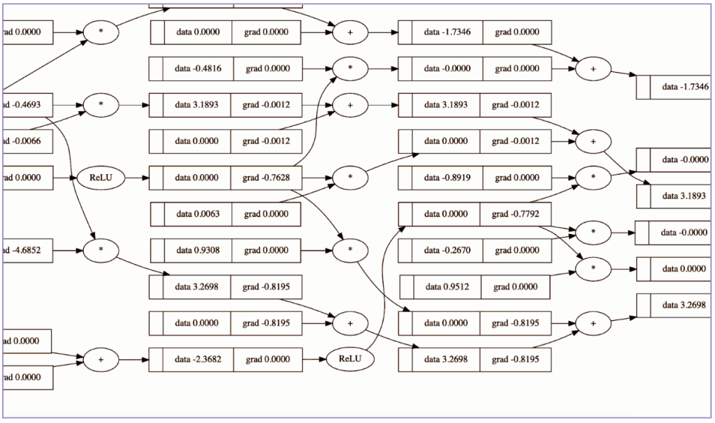
Even with a minimal MLP like the one from our example, we can see how the diagram is already getting more and more complex (too large to fit entirely within a readable screenshot). Not that anybody would want to for purposes other than learning, but one can imagine that manually doing these calculations would take a lot of time.

Lots of theory, code review and moving parts. Now is time to begin training our model.

Putting the Grad in Micrograd

As a quick recap, Loss measures how far the model’s prediction is from the correct answer. To reduce this Loss, the model uses backpropagation to compute how its parameters affect the amount of Loss, and then updates those parameters accordingly. This entire process is part of what is known as gradient descent.

Sticking to a Supervised Learning approach lets attempt to demonstrate how Micrograd automatically performs gradient descent. First, we provide our model with a small data set and its respective labels.

multi = MLP(2, [3, 3, 1])

a = Value(1.9)
b = Value(-1.1)
c = Value(2.1)
d = Value(-1.4)
e = Value(-1.6)
f = Value(-1.6)
g = Value(1.5)
h = Value(-1.3)
i = Value(0.8)

featrs = [[a, b, c],[d, e, f],[g, h, i]]
labls = [1.0, -1.0, 0.9]

We’ll use this Python code to say, “I want you to train on this data set” (i.e., the featrs) “and these are your goals” (i.e., the labls)

Every round of backpropagation and parameter adjustment that the model performs is aimed at making its predictions as close as possible to the actual label values. It does this by tweaking those of its parameters that interact with the provided input features.

If we run these bits and pieces of Micrograd as of now it will outputs some predictions:

model_prediction = [multi(value) for value in featrs]
model_prediction

[Value(data=0.2924872890061458, grad=0),
Value(data=0.37621014651628903, grad=0),
Value(data=0.30006197705162124, grad=0)]

Now the model needs a way to measure its performance. Let us define a Loss function and run these predictions through it.

loss = sum((yout - ygt)**2 for ygt, yout in zip(labls, model_prediction))
loss

Value(data=2.754454234971468)

Let’s trigger a backward pass and see pull the gradients for some of the parameters that took part in calculating such predictions.

loss.backward()

multi.parameters()

[Value(data=0.6733255363504393, grad=-1.0118017015874243),
Value(data=-0.23440127979473657, grad=0.8535407716931502),
Value(data=0, grad=-0.6960814851305541),
Value(data=0.24147437553736717, grad=0.02092726468125558),
Value(data=-0.7559823708639006, grad=0.6885323710707291),
Value(data=0, grad=-0.48410632904510437),
Value(data=0.018139230905912074, grad=-1.5783904539566305),
Value(data=-0.8441887534231638, grad=-1.3920366326349223),
Value(data=0, grad=0.8367013432646462), ..SNIP..]

These are the values that the model will adjust as part of training. The model will use the gradients at every step to guide its adjustments, but how exactly are gradients used to determine the optimal way of tweaking these parameters? 

Read the Gradient

If we pull a single parameter of our neural network model and its gradient, a weight value for example, we see that the gradient associated with this particular value is negative, which means the slope of the loss function is downward at that point.

single_weight = (multi.layers[0].neurons[0].w[0])
print(single_weight.data)
print(single_weight.grad)

0.6733255363504393
-1.0118017015874243

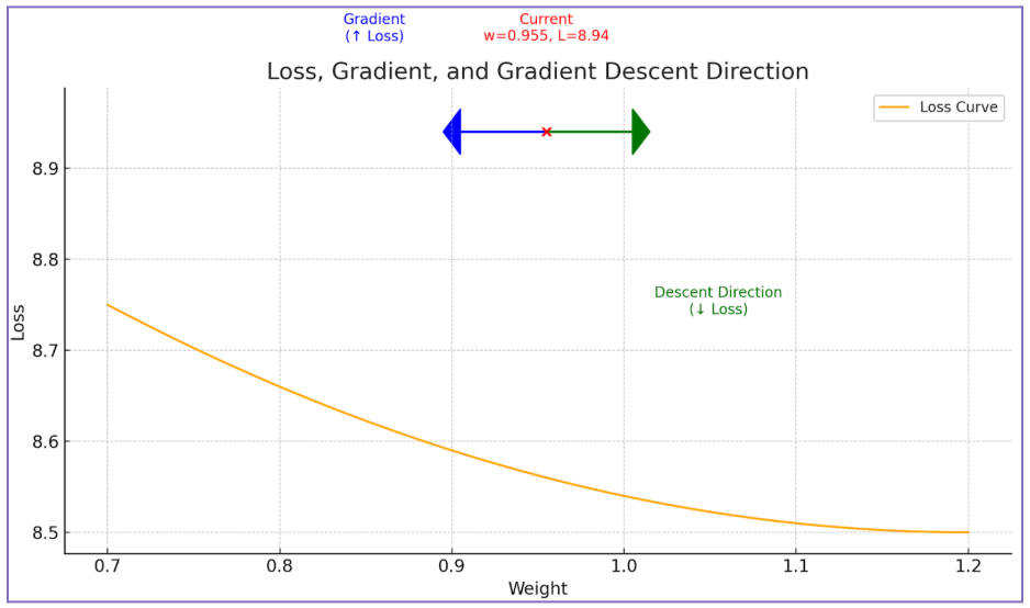
If we graphed the loss against the weight’s value, we’d observe that increasing the Weight lowers the Loss, nudging the Loss value downward on the graph.

In other words, the negative gradient tells us that making the parameter more positive moves us in the direction that reduces the Loss.

Here is another way to see it: the slope (or gradient) is pointing to the left, meaning the model can minimize Loss by shifting the Weight to the right plane, toward more positive values.

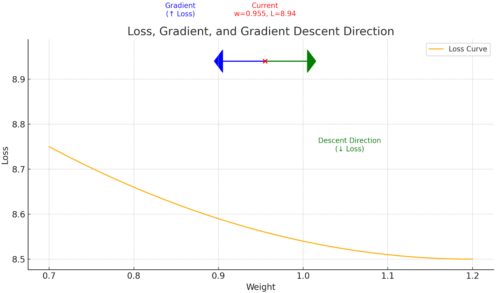
This concept might seem complex at first, but the key idea is simple: the gradient tells us the direction in which the loss increases (blue arrow). That is why in ML, and especially in gradient descent, we always want to move in the opposite direction of the gradient (green arrow) to reduce the loss.

Hyperparameters and Gradient Descent

From the theory section, not that this one lacks theory, but from the more theory-inclined section (pun intended), we learned that a model’s main hyperparameters are:

• Learning Rate
• Batch Size
• Epochs

Among these, the learning rate plays a key role during training. It controls how big a step the model takes when updating its parameters

Now that we understand that reducing Loss involves moving in the opposite direction of the gradients, we’ll use the learning rate in a function like the one shown below to perform that adjustment.

We ensure this by updating each parameter using this step, where:

• w is the weight being updated
  
• n is the learning rate (which controls how big the adjustment should be)
  
• We compute the update by multiplying the learning rate by the gradient of the weight (dL/dw) to determine how much and in what direction to adjust the weight.

Manual Adjustment Example

Let’s drill down on this adjustment step with a manual example. 

We’ll let our model make predictions using the training dataset we’ve defined, compare those predictions to their labels, and calculate the loss.

Previously, we pulled the gradient for a single parameter. Now, let’s use that gradient to implement an adjustment function and take one manual step of gradient descent.

Let’s implement the adjustment function and take a single manual gradient descent step.

single_weight.data += -0.1 * single_weight.grad
print(single_weight.data)

0.7745057065091818

This is a good sign for the model, because the gradient for that parameter was negative, meaning that increasing the Weight helps reduce the Loss. In other words, the model is learning that more of this value is beneficial for minimizing error in its predictions.

A model would repeat this adjustment step for every Weight it has. We can now observe this by wrapping these steps into a loop and letting it run for 10 iterations.

mlp = MLP(3, [3, 3, 1])

for n in range(10):

  # forward pass
  model_pred = [mlp(value) for value in featrs]
  #loss = sum((yout - ygt)**2 for ygt, yout in zip(labls, model_pred))
  loss = sum([(yout - ygt)**2 for ygt, yout in zip(labls, model_pred)], start=Value(0.0))

  # backward pass
  for param in mlp.parameters():
    param.grad = 0.0
  loss.backward()

  # update
  for param in mlp.parameters():
    param.data += -0.1 * param.grad

  print(n, loss.data)

By the third iteration, we observe that the loss has been reduced to 0.05781551259991121, meaning the model predictions are getting more accurate.

0 2.617980103561795
1 1.993278136288935
2 1.1921020869982601
3 0.5781551259991121
4 0.2958845244930379

Lower Loss value means the model is learning.

Outro

We have been able to observe model training single steps by following basic ML concepts and techniques while leveraging Micrograd. After these introductory concepts, ML grows in complexity, primarily to optimize the training process and produce models that aren’t limited to a single type of prediction.

Concepts like transformers, sentiment analysis, are some of the ones commonly seen in  following stages.

And again, I definitely recommend watching Andrej Karpathy’s walkthrough. There are a lot of other simple but cool details to Micrograd, like how it recursively iterates through the chain of operations as part of backprop or live troubleshooting some common mistakes seen in ML, which in this article does not cover.