Learning Machine Learning Part 2: Attacking White Box Models

In the previous post, I went through a very brief overview of some machine learning concepts, talked about the Revoke-Obfuscation project, and detailed my efforts at improving the dataset and models for detecting obfuscated PowerShell scripts. That resulted in three separate tuned models for obfuscated PowerShell script detection: a Logistic Regression model with L2/Ridge regularization, a LightGBM Classifier, and a 4-layer fully connected Neural Network. If you’re not familiar with machine learning, I highly recommend reading the first post before diving in here.

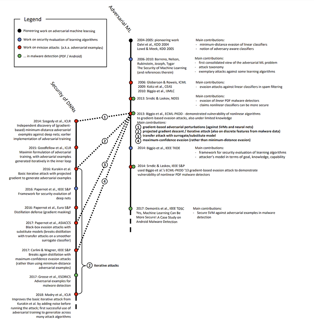
In this post I’m going to show how to attack these three models. This area of study is generally known as adversarial machine learning and is a fairly young discipline. While a 2018 paper by Battista Biggio and Fabio Roli points out that academic research on attacking machine learning goes back to at least 2004 with Dalvi et al., and the 2013 paper “Intriguing properties of neural networks” by Szegedy et al. showed some of the first adversarial examples for neural networks, the field didn’t start to really take off until around 2014 or so. The 2018 paper “Wild Patterns: Ten Years After the Rise of Adversarial Machine Learning” by Biggio et al. has a great timeline that documents the evolution of adversarial machine learning through 2018:

I’ve read a lot of (mostly academic) material on adversarial machine learning, and one of the seminal works of the field people often reference is the 2014 paper “Explaining and Harnessing Adversarial Examples” by Goodfellow et al. The attack algorithm described in that paper, known as the Fast Gradient Sign Method (FGSM) is one of the oldest practically implemented attacks in one of the most established adversarial machine learning toolkits, the Adversarial Robustness Toolbox.

This post will treat these models from a white box approach, where we have the entirety of the trained model itself including the input features, model architecture, and model parameters/weights. The third post in this series will tackle attacking these models from a black box perspective where only the input features are known, which is a more difficult problem.

I would be remiss if I didn’t mention all the work that Will Pearce (@moo_hax) has done in the last several years on adversarial machine learning in information security. His work was an inspiration for me to get started in this area, and a lot of the efforts I’m pursuing are iterations on his initial ideas.

The Jupyter notebooks described in this post are now updated in the Invoke-Evasion repository.

Adversarial Machine Learning

While adversarial machine learning is a relatively new discipline, there is a reasonable amount of material out there detailing research in this area. This used to be mostly academic, however, in the last few years practical frameworks have started that implement many of the attacks that previously existed only in whitepapers.

Unfortunately, most of the research appears to have been in the realm of image recognition. I believe the reason for this is likely because a) image classifiers are a very common application of machine learning and b) you can modify any pixel of an image by a small amount and still have the resulting adversarial image look like the original. The canonical adversarial image is is Figure 1 from “Explaining and Harnessing Adversarial Examples” by Goodfellow et al., often known as the panda example:

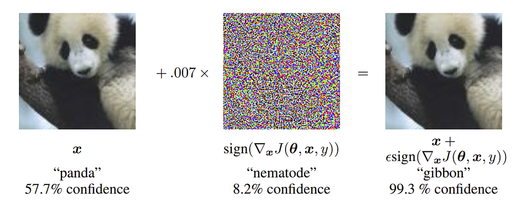
In the above example, an image originally classified as a panda has a specifically crafted set of adversarial “noise” applied to it (i.e., modifications to pixel values) that causes the new image to be classified as a gibbon, while the image still looks like a panda to human observers. While this is interesting and there are a lot of applications of image and video subversion in the real world, it’s definitely a different situation than what we’re dealing with in information security. For example, with the PowerShell script obfuscation problem space (and in fact many of our problems in infosec) we’re more limited in a) the number of features we can modify and b) to what degree we can modify said features. That is, we have a smaller functional subspace of modifications we can make to PowerShell scripts as opposed to images. I believe that this is a common scenario in information security focused machine learning models.

Also, likely as a consequence of adversarial research focusing largely on images, most academic literature assumes an attacker knows all the input features for a model. For images, this makes sense since the input features are pixels. For other examples, like our obfuscated script detection case study, this isn’t always the case. Feature extraction schemas can often be determined by reverse engineering, but for this post series I’ll assume we know all of the input features for simplicity. I hope to revisit this specific topic in future work.

Back to the type of attacks against machine learning algorithms. Will describes five general types of attacks against machine learning algorithms in several of his presentations:

Model Extraction is a fundamental adversarial ML technique that we’ll talk about in depth in the third post in this series. For this post, we’re going to focus on Evasion for the current white box models we already have.

I also want to differentiate between Adversarial Machine Learning and Offensive Machine Learning. Will defines Adversarial ML as the “Subdiscipline that specifically attacks ML algorithms” and Offensive ML as the “Application of ML to offensive security problems”, and I agree with these definitions. Adversarial ML is what we’re dealing with in this post series, where we’re crafting adversarial samples to evade existing models. Offensive ML would include things like sandbox detection, augmenting password guessing attacks, or improving spear phishing. This is an area that we’re exploring and we hope to have something to share soon!

Evasion

With evasion, there are generally two goals, somewhat analogous to strong and weak hash collision resistance. In one case we want any adversarial samples that are misclassified, and in the other we want to change the classification for a specific sample. These are known indiscriminate and targeted attacks respectively, sometimes termed misclassification and source/target misclassification.

Many well-trained machine learning algorithms are fairly robust to small amounts of random noise. With evasion, our goal is to add a small amount of specifically crafted noise to an input in order to change its classification label for a target sample. As Cody Marie Wild states in their “Know Your Adversary: Understanding Adversarial Examples” post, “The particular element that makes these examples adversarial is how little perturbation needed to be applied to get the network to change its mind about the correct classification.” In the traditional context of adversarial images, the goal is for the perturbed image to still look like the original image to a human observer, while having a different label from the model.

But first let’s back up a bit and talk about why evasion attacks against machine learning algorithms are even possible.

Adversarial Space

There’s a lot of academic research about this topic out there, but one of the best simplified explanations I’ve read is from chapter 8 “Adversarial Machine Learning” of Machine Learning and Security by Clarence Chio and David Freeman. The book describes the fundamental problem of imperfect learning- we aren’t able to provide a machine learning algorithm a “perfect” dataset that covers the entire input space for a problem. For example, we can’t provide all obfuscated and non-obfuscated PowerShell scripts for our examples from the first post. There’s also the case that the “irreducible error” might be non-zero, which is the error inherent to the training data that can’t be eliminated from any model. In this case, even if we eliminate imperfect learning, there are still adversarial samples that can result in misclassifications.

Figure 8–1 Adversarial space as a result of imperfect representation in training data from Machine Learning and Security illustrates this (emphasis mine):

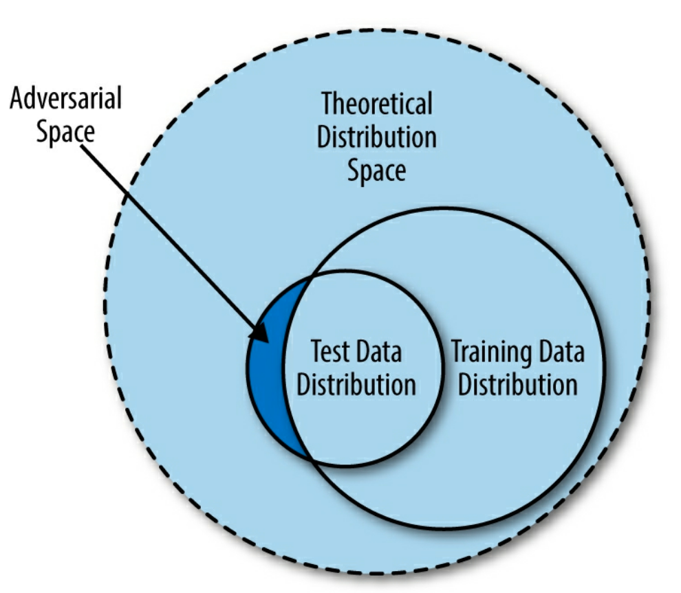
Essentially, the training data we provide a machine learning algorithm is drawn from an incomplete segment of the theoretical distribution space. When the time comes for evaluation of the model in the lab or in the wild, the test set (drawn from the test data distribution) could contain a segment of data whose properties are not captured in the training data distribution; we refer to this segment as adversarial space. Attackers can exploit pockets of adversarial space between the data manifold fitted by a statistical learning agent and the theoretical distribution space to fool machine learning algorithms.

Chio, Clarence; Freeman, David. Machine Learning and Security: Protecting Systems with Data and Algorithms . O’Reilly Media. Kindle Edition.

This post covers the evolution of theories for explaining adversarial samples. It also summarizes the “tilted boundary hypothesis” from this paper, which happens to match up well with the previous explanation:

In a nutshell, the authors argue that because the model never fits the data perfectly (otherwise test set accuracy would have always been 100%) — there will always be adversarial pockets of inputs that exist between the boundary of the classifier and the actual sub-manifold of sampled data.

The post also describes a 2019 paper from MIT that adversarial examples are a feature of how Neural Networks perceive data. Specifically, that adversarial examples are “a purely human-centric phenomenon”, as “robustness” is a human specified notion. As an admitted non-expert, I personally lean towards the tilted boundary hypothesis as described above. But the important point is that while there are competing theories about why adversarial samples are possible, for all machine learning systems there is an adversarial space that we as attackers may be able to exploit. Depending on our knowledge of the model architecture and internals, this exploitation is sometimes easier said than done.

White Box Versus Black Box

Most of us are familiar with the idea of a white box and black box perspective of a system. In machine learning literate, these terms have a slightly more specific definition. But first a (small, I promise) bit of math!

Remember back to the concept of a derivative in calculus:

TL;DR the slope of the above line is equivalent to the derivative of the graphed function at the red point. A gradient in machine learning refers to generalizing the derivative to three or more dimensions instead of the two shown here. So why do we care?

Because of gradient descent, an extremely important concept in machine learning.

As a very abbreviated explanation, the process for finding the “optimal” internal configuration for many (but not all) machine learning algorithms is as follows:

1. Plot all of your training data points in N-dimensional space. For example, if you have 1000 samples and 14 features, you plot those 1000 samples in 14-dimensional space. Don’t try to visualize it, you can’t. To quote Geoffrey Hinton, “To deal with hyper-planes in a 14-dimensional space, visualize a 3-D space and say ‘fourteen’ to yourself very loudly. Everyone does it.”
2. Initialize a random hyperplane — a line to 2-dimensional space is to a hyperplane in higher-dimensional space.
3. Run a number of samples through the model, and measure how correct/incorrect each prediction is using a loss function, also often referred to as the error function. This just tells you how off or accurate the model’s prediction was. A common example is log-loss, also known as cross-entropy loss.
4. Use the gradient of the loss function to tell you where to nudge the internals of your model in order to minimize the loss. This gives you information about in which direction to nudge these internals, and by how much.
5. Repeat this process until you hit some kind of stopping criteria, resulting in a (hopefully!) reasonably optimized model.

The real process is more complicated than this but that’s the general idea- you have a loss function that tells you how incorrect your current model internals are, and you use the gradient of this function to intelligently guide how you’re adjusting model internals in order to minimize the prediction mistakes on training data.

Sidenote: one of the big exceptions are tree ensembles like Random Forests and Gradient Boosted Decision Trees, as they are non-continuous step functions that don’t have a gradient. This means that most of the efficient white box adversarial attacks out there will not work against these architectures, though some black box attacks can be effective. There is some research on attacking tree ensembles but that research area is generally not as robust as the adversarial work against models with gradients

Back to the white box and black box perspective. In adversarial machine learning, a white box attack is one where we know everything about the deployed model, e.g., inputs, model architecture, and specific model internals like weights or coefficient values. In most cases this specifically means that we have access to the internal gradients of the model. Some researchers also include knowing the full training data set in white box attacks, but this is not always necessary for evasion. Conversely, a black box attack is one where we only know the model inputs and have an oracle we can query for output labels or confidence scores.

Evasion in adversarial ML can be thought of as gradient ascent instead of gradient descent — we want to increase the loss for one or more samples instead of decreasing it. We can also think of adversarial ML as a type of max-min problem. We want to maximize the error for one or more samples while minimizing the changes we make to the sample (also known as adversarial perturbations).

White box attacks are generally more effective than black box attacks at this task because we can use the internal model gradients to more accurately perform the gradient ascent process versus a black box approach. This makes it faster and more efficient to calculate the minimum change needed to create an adversarial sample.

Interpretability

In our concept, interpretability or explainability involves how well a human can understand why a model makes a particular decision. Why does this matter for evasion? Well not all features in a machine learning model are equally influential. If we can gain information about which features have the most impact on a model’s decision boundary, we can use this insight to guide our evasion process.

As Christoph Molnar states in his Interpretable Machine Learning book (a great, but dense, read by the way), “Interpretability might enable people or programs to manipulate the system.” We’ll show how interpretability can be used as an evasion tool In the Evasion Method A — Feature Importance Extraction and Manual Modification section of this post.

Invoke-Evasion Problem Statement

We have three models from our first post that take 446 features measured from the abstract syntax tree (AST) of a PowerShell script and return a label of obfuscated or normal. We also have a script that’s currently classified as obfuscated, and we want to modify it so a given model misclassifies the sample as normal.

Thinking through this problem, with each model we have a hyperplane through 446 dimensional space that divides the points of our sample sets, where our malicious sample is a point currently residing on the obfuscated side of the decision boundary. We want to modify one or more properties of the script so we preserve the functionality of the script (and obviously retain its obfuscated “nature”) but we move the data point for the script across the decision boundary to normal, ideally with the least amount of modification possible.

Let’s look at two ways to do this- extracting feature importances in order to perform manual modification, and using established attack algorithms against our models.

Evasion Method A — Feature Importance Extraction and Manual Modification

Before we can make any modifications to an obfuscated script, we want to know which features in each model influence the final classification decision the most. Here is where the explainability or interpretability issue I keep mentioning comes into play. Our three models have increasing levels of complexity which increases the difficulty explaining which features matter the most.

Logistic Regression

With Logistic Regression being a linear model, explainability is easy. A Logistic Regression takes the following form:

Or in another, more common form:

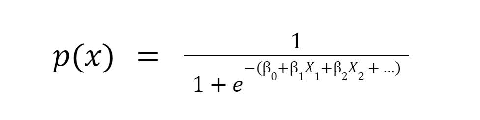
The reason we like this function is that it bounds the output between 0 and 1, making it great for classification tasks. An example curve for the standard Logistic Regression is:

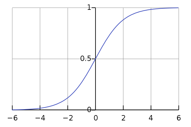
Don’t be scared by the above formulas! Let’s see how this works.

To classify a sample, each measured feature value for a script (Xᵢ) is multiplied by an associated fixed weight/coefficient (Bᵢ), a bias is added (B₀), and the value is input for X in the standard logistic formula f(x) = 1 / (1 + e^-x), also known as the Sigmoid function. A Logistic Regression is considered linear in nature because it uses a linear combination of the input variables (B₀+B₁X₁+B₂X₂+ … ) which makes it fairly interpretable for us. The larger a feature’s weight/coefficient, the more that feature influences the final decision of the model. The sign of the feature (+/-) determines which label the feature is pushing towards. The exact amount the feature contributes is defined by “log-odds”, which I won’t get into here because:

But if you are interested in the exact interpretation of Logistic Regression coefficients (I mean, who isn’t?) knock yourself out.

So if we want to push our script over the decision boundary to flip a label from obfuscated (1) to normal (0), we need to know which features contribute most towards the obfuscated label and which contribute most to the normal label. In mathy terms, we want to know which coefficients had the largest absolute value for both the positive and negative direction.

Let’s see how this compares for both the original Revoke-Obfuscation Logistic Regression model and then our tuned Logistic Regression model.

Original Revoke-Obfuscation Logistic Regression

The original Logistic Regression model from the Revoke-Obfuscation work is encapsulated here, with the first term being the intercept/bias. Since we have all of the inputs and model parameters, this is a complete white box scenario. We want to know which features influence the model the most towards obfuscated and normal, so let’s evaluate the model on a known script so we can easily get the feature names, match those features up to the coefficients (e.g., Bₓ) in $highConfidenceWeightedVector from Revoke-Obfuscation, and select the top 10 and bottom 10 coefficients by value:

$Vector = Get-RvoFeatureVector -Path C:ToolsPowerView.ps1

$FeatureNames = $($Vector.Keys)

[System.Double[]] $highConfidenceWeightedVector = @(-218.9926, -4217.0000, …))

$Features = for ($i = 0; $i -lt $($Vector.Count); $i++) {

$Feature = New-Object -TypeName PSObject

$Feature | Add-Member -MemberType NoteProperty -Name “Feature” -Value “$($FeatureNames[$i])”

$Feature | Add-Member -MemberType NoteProperty -Name “Value” -Value ([float]($highConfidenceWeightedVector[$i+1]))

$Feature

}

$Features | Sort-Object -Property Value -Descending | select -first 10 -Last 10

…

We get the following result:

The positive values contribute the most towards 1, meaning obfuscated, and the negative values contribute the most towards 0, meaning normal. Let’s check out what the AstStringMetrics_CharacterDistribution_/_2f_Count feature means by checking out the Revoke-Obfuscation source for this check here and here. It looks like this check extracts all string constants from the script’s Abstract Syntax Tree (AST), and returns the total number of 0x2F (which translates to “/”) characters across all constants in the script. According to Microsoft, “This includes both single and double quoted strings…” So what will happen if we create a new string consisting of “/”s, and stuff it into a script previously measured as malicious, like the DBOdemo1.ps1 script?

Original DBOdemo1.ps1 script:

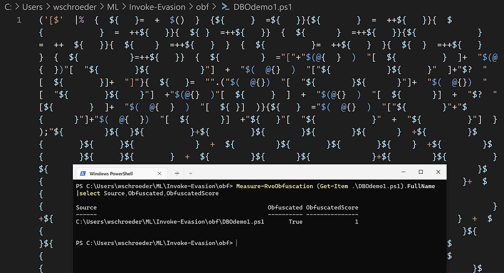
Modified DBOdemo1.ps1 script:

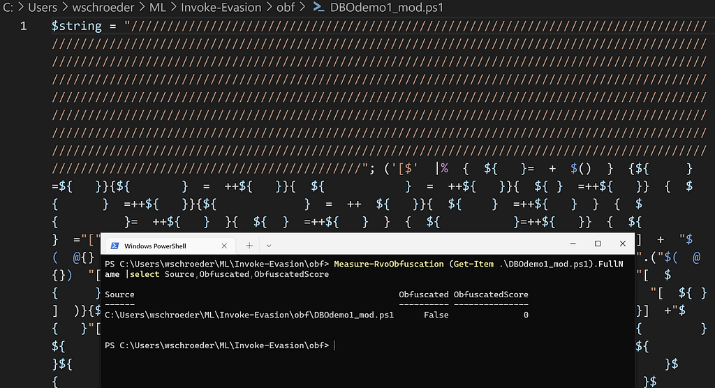
Awesome! Note that we could have done this with most of the large negative coefficients, but smaller magnitude terms would have taken more “/”s. Now let’s turn our attention to our tuned Logistic Regression from the first post.

Sidenote: we’ll continue to use the DBOdemo1.ps1 script as a benchmark for all attacks in this post series.

Tuned Logistic Regression

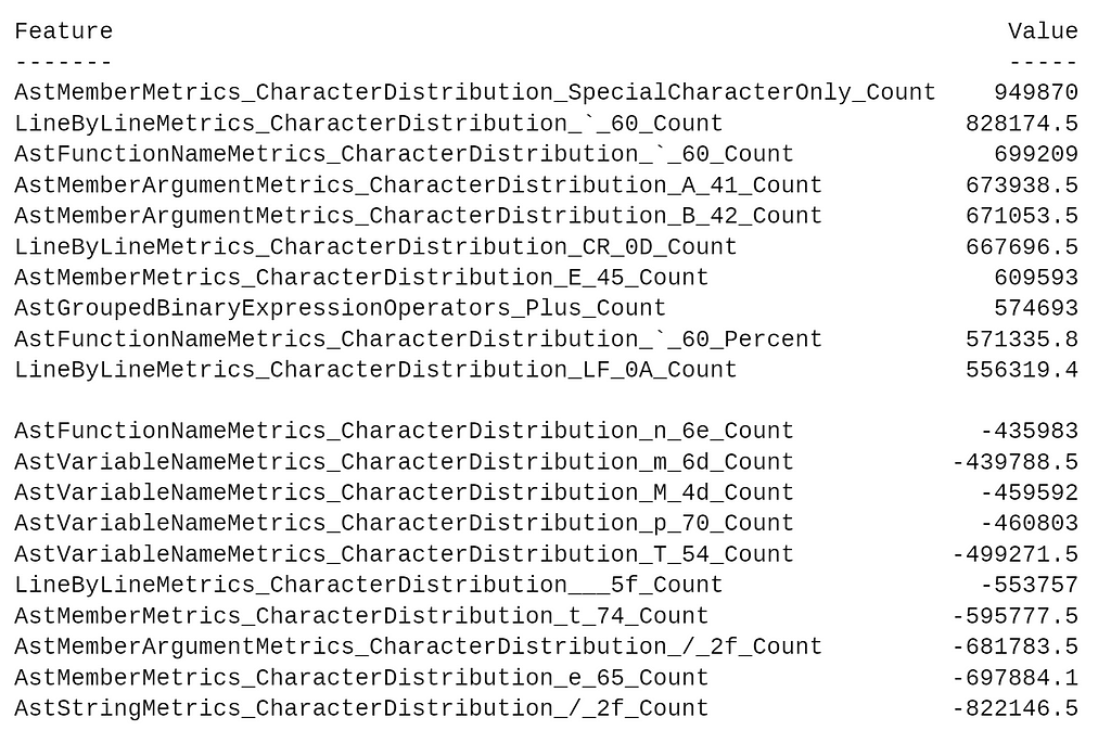
Remember from the first post that our tuned Logistic Regression uses the 446 features selected from Boruta-Shap and we ended up with a penalty of L2 (Ridge), C of 5, and a saga solver. Let’s load up the saved model, and zip up the feature names with the coefficients. Then we’ll sort the features by value, and output the top and bottom 10 (see the WhiteBox.ipynb notebook in the Invoke-Evasion repo for details).

The results are:

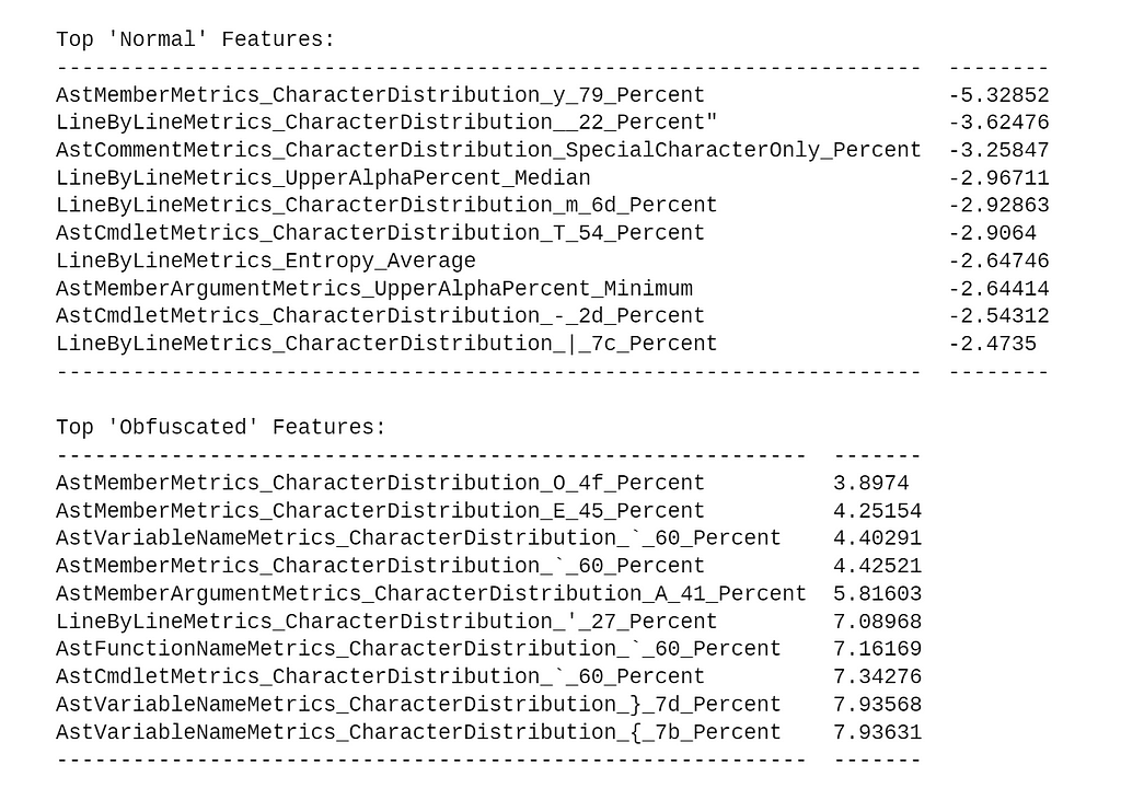
Looking at the above table, it’s interesting that we end up with different features than the original Revoke-Obfuscation model. We’ll revisit this and why it matters in the third post in the series.

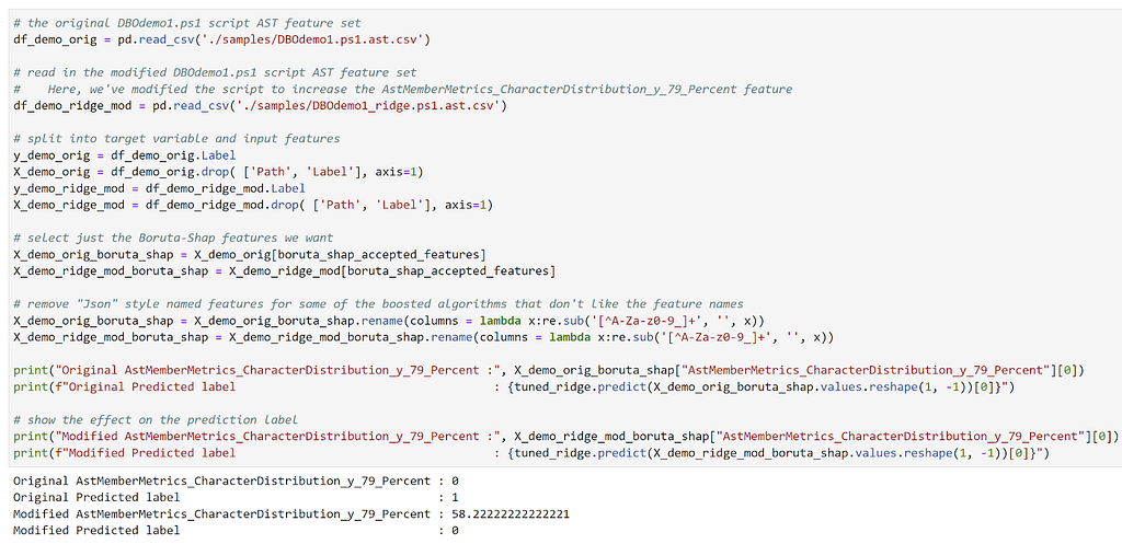
Again, the positive values contribute the most towards 1, meaning obfuscation, and the negative values contribute the most towards 0, meaning normal. In this case, the AstMemberMetrics_CharacterDistribution_y_79_Percent feature has the most influence towards the normal label. According to Microsoft, “The ast that represents accessing a member as a property, e.g. $x.Length or [int]::MaxValue.” So let’s try accessing a non-existent property containing a bunch of y’s (0x79) for some variable. Hopefully this raises the percentage up and helps that feature move the sample over the decision boundary:

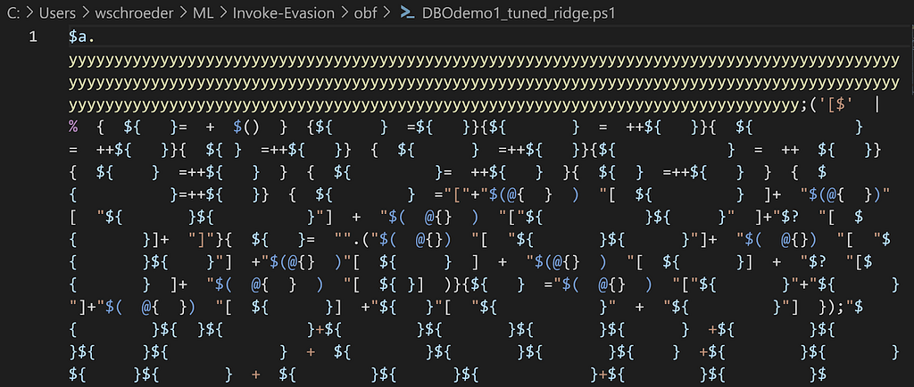
Success! If we add enough y’s to the property we’re accessing, we’re able to move the label for this very obfuscated script to the normal boundary.

LightGBM feature_importance

As I mentioned in the first post, tree ensembles like Random Forests and Gradient Boosted Decision Trees inherently contain the importance of how “important” the feature is. This post has a good summary as to why:

…when training a tree, it is possible to compute how much each feature decreases the impurity. The more a feature decreases the impurity, the more important the feature is. In random forests, the impurity decrease from each feature can be averaged across trees to determine the final importance of the variable.

It also has a simplified explanation as well:

…features that are selected at the top of the trees are in general more important than features that are selected at the end nodes of the trees, as generally the top splits lead to bigger information gains.

These aspects also hold true for boosted trees, like our LGBMClassifier model. This is the exact problem that Adrian Kress explored in his excellent “Evading Static Machine Learning Malware Detection Models — Part 2: The Gray-Box Approach” which I highly recommend everyone read. As Adrian describes in the post, there are two main approaches here: split and gain.

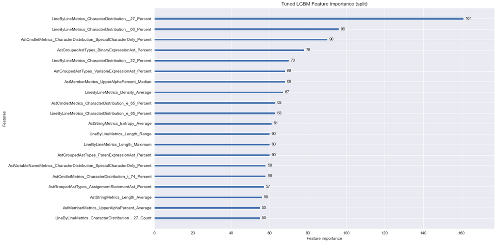
Using LightGBM’s plot_importance function with feature_importance=split, we can determine the most used features in our model:

Using feature_importance=gain, we can determine the features that have the highest impact on the obfuscated vs normal label if the feature is used at least once:

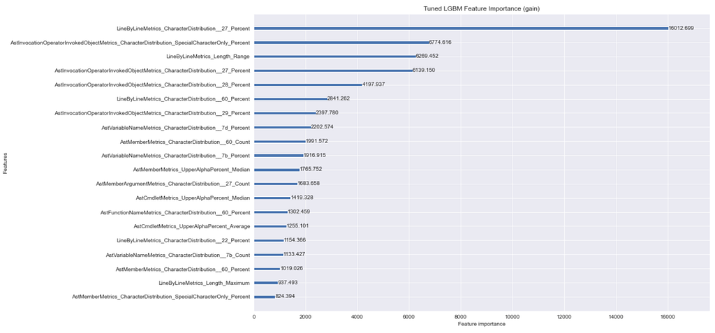
Looking at these two plots, a lot of these results make sense. Specifically, the LineByLineMetrics_CharacterDistribution__27_Percent feature (our JSON feature name encoding removed the ‘) matters a lot. This makes sense considering the single quote is used in a lot of obfuscated PowerShell samples.

Since we want to preserve the original obfuscated script as much as we can, we want to add things that influence “normal” metrics instead of removing things like single quotes or backticks. One downside of feature importance plots is that they don’t let you know in which direction the feature influences the decision, so we have to make some assumptions. The AstMemberMetrics_CharacterDistribution_e_65_Percent feature seems like something that’s more common in normal scripts. Let’s add a bunch of e’s to a variable the similar to what we did previously and see if we can move the boundary:

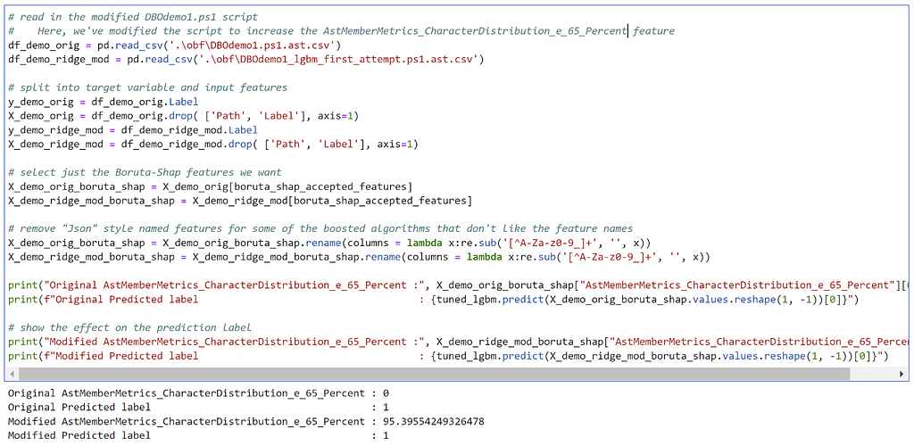
No dice. Tree ensembles — like Random Forests and Gradient Boosted Decision Trees — appear to be, at least in this case, much more robust against evasion. This is something that others have observed as well in at least some cases.

So is all hope lost?

LightGBM SHAP

Enter SHapley Additive exPlanations, usually referred to as SHAP, a “game theoretic approach to explain the output of any machine learning model.” While I won’t get into a technical explanation of what SHAP is (there are other resources already available for that), I will show how we can use SHAP to derive some insight into the LightGBM model we’re targeting.

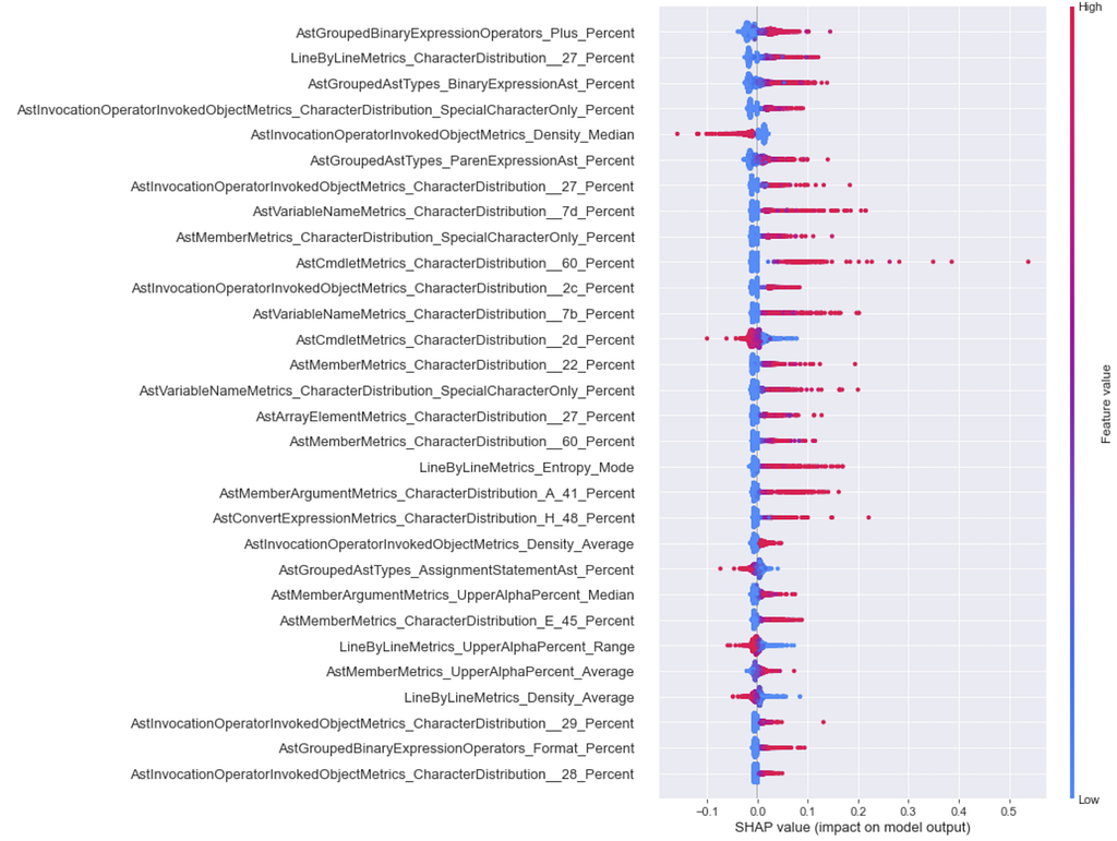
One thing I want to briefly touch on before diving in is the concept in SHAP of global interpretability versus local interpretability. The global interpretability insights provided by SHAP can show how much each feature contributes to a model’s output, in this case obfuscated or normal, across the entire data set. There are a few ways to do this, but my preferred method is the summary_plot (or beeswarm plot). The example beewarm for all features in our LightGBM model is:

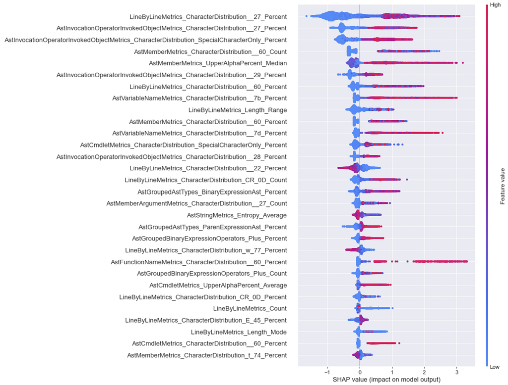
Features in this plot are ranked in descending order of importance, that is, features that have a higher impact on the model’s output are higher up the plot. The x-axis represents the SHAP value for a feature, where a higher SHAP value means that the model is more likely to return a model label of 1, or obfuscated in our specific situation. Red means that the feature value is high, and blue means the feature value is low. So looking at this plot, we can see insights that make sense, like having a low percentage of single quotes (hex 0x27) line by line is associated with a normal label. For more detail on interpreting this type of plot, check out this StackExchange post or this section in Interpretable Machine Learning.

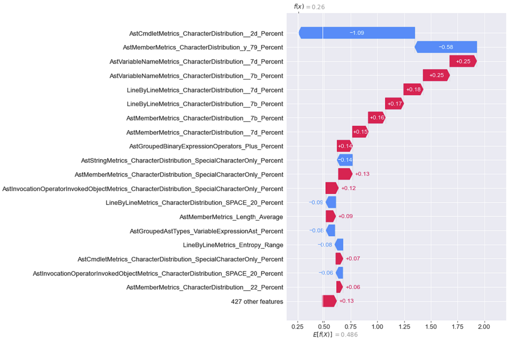
Local interpretability means that SHAP can show us which features contributed the most to a specific sample’s classification rather than feature effects across all samples. This can be done with waterfall and/or decision plots. The Jupyter notebooks for all this show both, but I’ll just highlight the waterfall plots here.

My approach for this particular case was to use insights from the global beeswarm plot for the model to to pick normal features from to iteratively add to the script. After each modification I regenerated the waterfall plot for the sample to see the effect of the change.

Here’s the waterfall for the features from the original DBOdemo.ps1 script before modification:

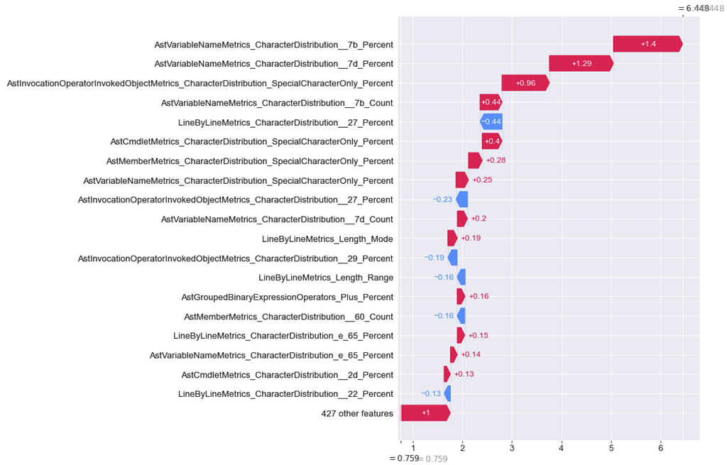
The above plot shows features in red that pushed the decision towards obfuscated, and features in blue that pushed the decision towards normal. In this case, we want to modify features to push that top number (6.448) to negative territory.

I then made repeated modifications to the sample, trying to minimize any features that pushed the sample to obfuscated and maximize any features that pushed the sample to normal. After each process extracted the features again for the modified script and regenerated the plots, repeating this process until the sample moved across the boundary:

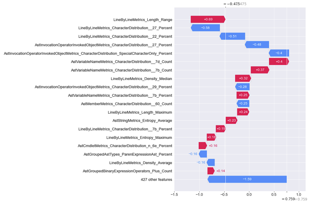
There were a lot of modifications, significantly more than what was needed to evade the Logistic Regression model. Obviously there are more efficient adversarial modifications for this sample than what I did here, this was just a first (but not optimized) attempt. As I previously mentioned, the robustness of tree ensembles has been observed by others as well. While there has been some recent work on specifically attacking tree ensembles it’s still dwarfed by adversarial work against Neural Networks.

Sidenote: this isn’t always the case! Adrian Kress was able to heavily evade a LightGBM model trained on the EMBER dataset by examining feature importances and just changing the timestamp for a malware sample. Every dataset and model are different!

Neural Network

Neural Networks are not inherently explainable like Logistic Regression or tree ensembles are. Our main option is to use something like SHAP, so let’s get to it with global feature importances in a beeswarm:

We don’t get quite as good results as we did with the SHAP TreeExplainer, because for Neural Networks the conditional expectations of the SHAP values are approximated using a number of background samples instead of the entire dataset. In English: for deep learning models, a random subset of samples are used with math to approximate SHAP values, while exact SHAP values can be calculated from tree based models. Regardless, the above figure does give us some idea as to which features push things towards normal.

We’re going to repeat the process we used to attack the LightGBM model, where we generate waterfall/decision plots for a sample we’re trying to modify, make our modifications, extract the features and regenerate the plots until we cross the decision boundary. Here’s where we start with our example:

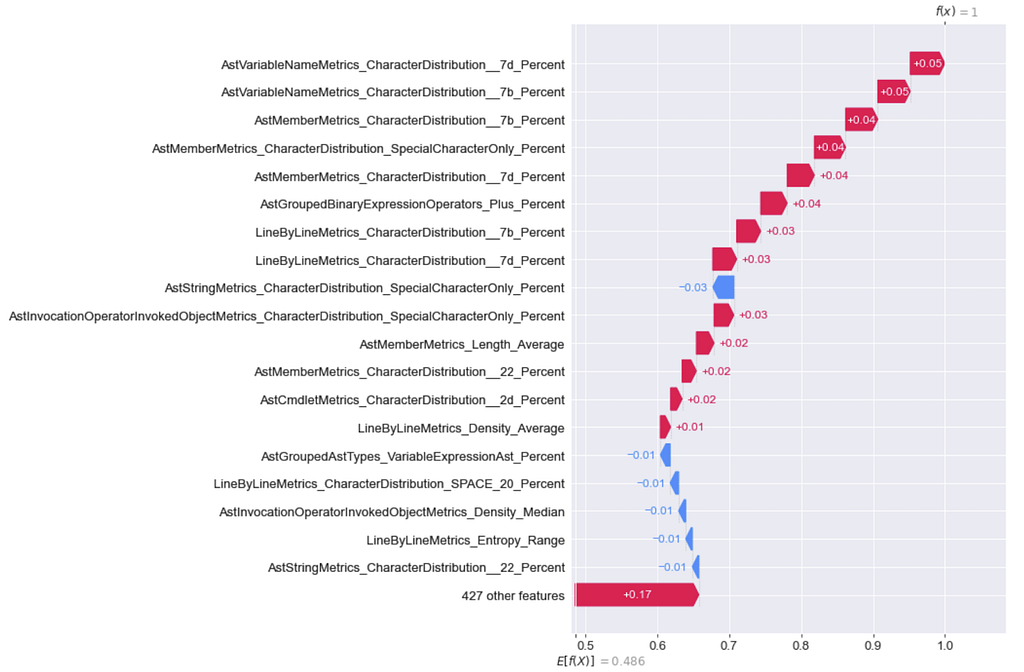
And after only a few modifications, here’s what we get:

Specifically, this is all I added to the top of DBOdemo.ps1:

function t — — — — — — — — — — — — — — — — — — — — — — — — — a{}

t — — — — — — — — — — — — — — — — — — — — — — — — — a

$a.yyyyyyyyyyyyyyyyyyyyyyyyyyyyyyyyyyyyyyyyyyyyyyyyyyyyyyyyyyyyyyyyyyyyyyyyyyyyyyyyyyyyyyyyyyyyyyyyyyyy

…rest of DBOdemo.ps1…

This Neural Network model ended up being significantly easier to evade than the LightGBM model, at least in this case. Remember that every dataset and model are differentʸᵒᵘʳ ʳᵉˢᵘˡᵗˢ ᵐᵃʸ ᵛᵃʳʸ.

As far as feature importance and SHAP goes, there are some commonalities between the models like {}’s, backticks, and single quotes usually showing up in some form. However, the most “important” features for each model vary. This often happens in machine learning when the data set is relatively “noisy”- each model narrowed in on a different subset of features that proved effective. This will have implications for the third post in this series when we attack these models as a black box.

Evasion Method B — Common Attack Algorithms

I mentioned in the first part of this post that there has been a good amount of work over the past 8 years or so on the academic side of machine learning. More recently, practical frameworks have started to emerge that allow us to actually execute many of these attacks. One of the most established, general purpose frameworks is the Adversarial Robustness Toolbox (ART), which we’ll be using in this post.

I also previously mentioned how much of the academic research has been around adversarial images, and the evasion attacks implemented in ART reflect that. However, like we covered, we have a smaller functional subspace of modifications we can make to PowerShell scripts versus images. My theory was that we’d ideally want an attack algorithm that lets us specify which specific features we want to perturb (known as feature masking) when generating adversarial examples. Luckily, these algorithms in ART allow us to do this:

• Projected Gradient Descent (PGD, white box)
• Auto Projected Gradient Descent (Auto-PGD, white box)
• Fast Gradient Method (FGM, white box)
• HopSkipJump (HSJ, black box) — “HopSkipJump is basically the pass-the-hash of Adversarial ML.” — Will

PGD, Auto-PGD, and FGM are white box attacks that rely upon knowing the internal model gradients to generate adversarial samples. Because decision trees and tree ensembles don’t have an explicit gradient, other white box techniques are needed to attack them. Most attack examples against tree ensembles I’ve seen use black box methods such as HopSkipJump or Zeroth Order Optimisation (ZOO) — there is a specific Decision Tree attack algorithm in ART, but it doesn’t work against tree ensembles like Random Forests and Gradient Boosted Trees. Because of these restrictions and because I could not get Auto-PGB to work with my models correctly, I used PGD, FGM, and HSJ on the Logistic Regression as an example.

The WhiteboxBox.ipynb Jupyter notebook in the Invoke-Evasion repository has all of my attempts and results for this section, but for the sake of brevity I’m just going to summarize the approach and results here.

First off, which subset of features do we want to aim to modify? My theory was that the easiest options that preserve the original script’s functionality are metrics that involve character counts, like AstVariableNameMetrics_CharacterDistribution_E_74_Count. The other advantage is that while many of the feature metrics are percentages, which limits their range to 0–100 in a practical scenario, there isn’t a limit to how much we can increase *_Count features.

I took the tuned Logistic Regression algorithm and extracted all the feature weights that are negative, meaning they push the model decision towards normal. I then filtered down those for *_CharacterDistribution_X_Count type metrics resulting in 16 target features which I used to build a feature mask. For each attack algorithm I generated adversarial samples using both the feature mask to modify only the features I specified, as well as generating samples using no feature masking at all.

Somewhat surprisingly, the black box HopSkipJump attack produced significantly better masked adversarial results than Projected Gradient Descent or the Fast Gradient Method. I assumed that a white box method with knowledge of the model’s internals would fare better, but I’m guessing that I likely messed up the processing for feature scaling somehow (see the Jupyter notebook for more details). However none of the results were super promising.

But even if an attack algorithm is able to successfully modify a subset of our features with relatively minimal changes, there’s still a pretty big elephant in the room: how do we actually use these adversarial numbers the attack algorithms generate?

That is, if we are actually able to modify the tabular feature measurements for a sample to change its classification label, how do we map those modified numbers back to an actual script in a way that the script still functions as originally intended. Specifically, what is the ??? process here:

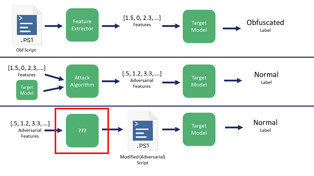
Fear ye not, there is a solution to this problem that I’ll cover in the third post in this series.

Conclusion

If you have a complete model you can derive a lot of insight about its decision process against specific samples. In our case we were able to use these feature importances to guide our manual evasion for the obfuscated DBOdemo.ps1 sample script. While SHAP was built for model explainability, we used it here to manually craft adversarial samples efficiently, an approach that is potentially novel.

In this particular case study, manually crafting adversarial samples against white box Logistic Regression models was significantly easier than crafting samples against tree ensembles like Random Forests or Gradient Boosted Trees, but only marginally easier than against Neural Networks. This generally makes sense due to the linear nature of Logistic Regression. If I were to use one of these three models in production similar to Joost Jansen’s approach in “Machine learning from idea to reality: a PowerShell case study”, I would choose the Gradient Boosted Decision Tree. This architecture proved to be not only the most accurate but also the most resilient against evasion attacks for this particular application. These results are not guaranteed for all applications: data is weird.

As far as attack algorithms like HopSkipJump go, a big challenge we have with this specific script obfuscation scenario is how we can take an adversarial sample generated from something like HopSkipJump and map those feature modifications back to an actual sample script. While this is how these attack algorithms have traditionally been used, there is another way of looking at the problem that I’ll detail in the next post in this series.

All of these issues aside, models are vulnerable. It’s just a question of how vulnerable they are and how much effort it takes to subvert them. In the next post we’ll examine attacking these three models from a black box perspective where the model architectures are not known.

The Jupyter notebooks described in this post are now updated in the Invoke-Evasion repository.

References

• SHAP
• The Adversarial Robustness Toolbox
• These two posts by Adrian Kress on evading machine learning malware models, which were a great inspiration
• The “Machine learning from idea to reality: a PowerShell case study” post by Joost Jansen
• Interpretable Machine Learning by Christoph Molna
• All of Will Pearce’s talks

---

Learning Machine Learning Part 2: Attacking White Box Models was originally published in Posts By SpecterOps Team Members on Medium, where people are continuing the conversation by highlighting and responding to this story.