Learning Machine Learning Part 3: Attacking Black Box Models

In the first post in this series we covered a brief background on machine learning, the Revoke-Obfuscation approach for detecting obfuscated PowerShell scripts, and my efforts to improve the dataset and models for detecting obfuscated PowerShell. We ended up with three models: a L2 (Ridge) regularized Logistic Regression, a LightGBM Classifier, and a Neural Network architecture.

The second post covered attacking these models from a white box perspective, i.e., where we have the entirety of the trained model itself including the input features, model architecture, model parameters/weights, and training data. I highly recommend at least skimming these first two posts before proceeding to ensure this all makes as much sense as possible.

In this post we’re going to cover the more common, and difficult, black box perspective. Here we only know what features are being extracted from each sample – even the architecture will remain opaque to us.

Background

After reading what was definitely hundreds of pages of academic research on adversarial machine learning, I can safely say that a good chunk of the research has been from a white box perspective. Remember our definition of white box and black box attacks from the second post in this series:

• A white box attack is one where we know everything about the deployed model, e.g., inputs, model architecture, and specific model internals like weights or coefficients.
• A black box attack is one where we only know the model’s inputs, and have an oracle we can query for output labels or confidence scores. An “oracle” is a commonly used term in this space that just means we have some kind of an opaque endpoint we submit our inputs to that then returns the model output(s).

Also, most of the research appears to have been in the realm of image recognition. While this is interesting, it’s definitely a different problem space than what we’re dealing with. Specifically, images can have multiple pixels perturbed by a small amount without the resulting adversarial image appearing to be modified to the human eye. For a lot of the problems we’re dealing with in security, for example our PowerShell obfuscation problem space, we’re more limited in a) the number of features we can modify and b) to what degree we can modify said features. That is, we have a smaller functional subspace of modifications we can make to PowerShell scripts as opposed to images.

A number of black box attacks involve model extraction (see the next section) to create a local model, sometimes known as a substitute or surrogate model. Existing attacks are then executed against the local model to generate adversarial samples with the hope that these samples also evade the target model. This often works because of the phenomenon of attack transferability, which we’ll talk about shortly.

Black box attacks can also skip model extraction and directly query inputs against the target model. These attacks, where the internal configuration of the model is not needed at all, are what’s actually known as black box attacks in the academic literature. However, by using model extraction we can potentially apply white box attacks against local clones of black box models where we only have an oracle to submit inputs to and get labels from.

Model Extraction

Model extraction, according to Will Pearce and others, is one of the most fundamental primitives in adversarial ML. While this idea was likely around for a while, I believe the first formalizations of model extraction (or at least one that popularized the method) were the 2016 paper Transferability in Machine Learning: from Phenomena to Black-Box Attacks using Adversarial Samples” and the 2017 paper “Practical black box Attacks against Machine Learning” both from Papernot et al. The general summary of their approach from the 2017 paper is:

Our attack strategy consists in training a local model to substitute for the target DNN [Deep Neural Network], using inputs synthetically generated by an adversary and labeled by the target DNN. We use the local substitute to craft adversarial examples, and find that they are misclassified by the targeted DNN.

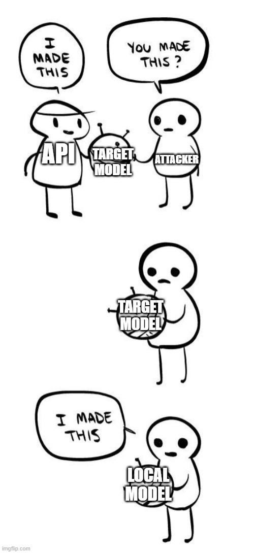
The entire idea is to approximate the target model’s decision boundary with less (and usually different) data than the model was originally trained on. Basically, model extraction involves first submitting a number of known labeled samples to the model, which functions as a labeling oracle. Imagine submitting a bunch of binaries to some kind of website that lets you know whether the binaries are malicious or not. Or imagine having our adapted Revoke-Obfuscation models as some kind of internal API, where we can submit our feature measurements and get a label result of normal or obfuscated, or a probability-of-obfuscation score. With enough inputs, we can train a local substitute model that functions similarly to the target model.

Figure 1 from “Active Deep Learning Attacks under Strict Rate Limitations for Online API Calls” by Shi et al. summarizes the process well:

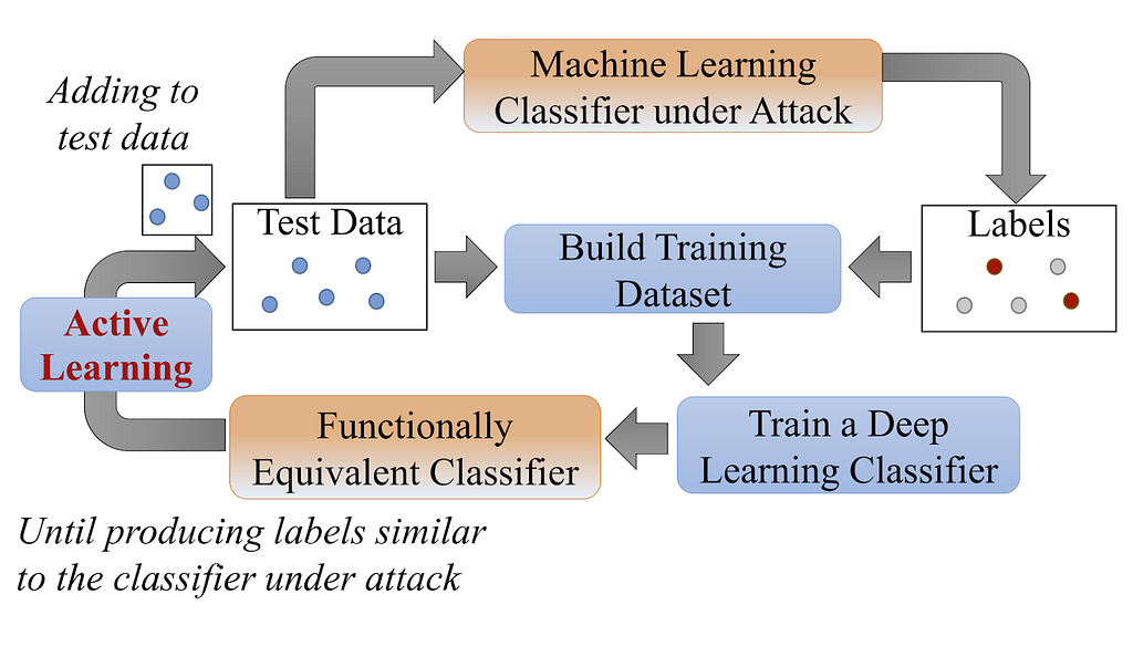
A reasonable hypothesis is that the closer we can match the original model architecture, the better our local model will function. This is something we’ll be exploring in this post.

A slightly different approach involves training an initially poor model with few samples, and using some of the white box attack techniques described in the second post to generate adversarial samples. These samples are run through the classifier, and as described by this post:

…the adversarial examples are a step in the direction of the model’s gradient to determine if the black box model will classify the new data points the same way as the substitute model. The augmented data is labeled by the black box model and used to train a better substitute model. Just like the child, the substitute model gets a more precise understanding of where the black box model’s decision boundary is.

End result either way? We have a locally trained model that approximates the target model’s decision boundary. With this, we can perform various white box based attack algorithms that exploit internal model gradients, in addition to any black box attacks as well.

Sidenote: Inputs and Model Architectures

If the inputs to the model you’re attacking are images or text, in some ways you’re in luck as you can likely guess the target model base architecture. There are established guidelines for these types of inputs i.e., Convolutional Neural Networks for images and LSTM/Transformers (or Naive Bayes in specific cases) for text. In these examples, we’re going to work with tabular data, meaning data that is displayed in columns or tables. We’ll hopefully revisit attacking text-based models another time!

Attack Transferability

You might be asking, “Really? Attacks against crappy locally cloned models can work against real production models?” The answer is YES, due to a phenomenon called attack transferability. The 2019 paper “Why Do Adversarial Attacks Transfer? Explaining Transferability of Evasion and Poisoning Attacks” by Demontis et al. explores this from an academic point of view, but I’ll do my best to explain the concept. Also, considering that this paper is only a few years old and there’s not a general consensus as to why adversarial attacks transfer, remember that this is still somewhat of an open question.

The seminal work that introduced this concept is the previously mentioned 2016 paper “Transferability in Machine Learning: from Phenomena to Black-Box Attacks using Adversarial Samples” by Papernot, McDaniel, and Goodfellow. The first few sentences from the abstract give a good overview of the concept (emphasis mine):

Many machine learning models are vulnerable to adversarial examples: inputs that are specially crafted to cause a machine learning model to produce an incorrect output. Adversarial examples that affect one model often affect another model, even if the two models have different architectures or were trained on different training sets, so long as both models were trained to perform the same task. An attacker may therefore train their own substitute model, craft adversarial examples against the substitute, and transfer them to a victim model, with very little information about the victim.

Their paper sets out to prove two hypothesis, namely that “Both intra-technique and cross-technique adversarial sample transferabilities are consistently strong phenomena across the space of machine learning techniques’’ and that “Black-box attacks are possible in practical settings against any unknown machine learning classifier.” Their paper makes a compelling case for each, and also demonstrates the transferability of different model classes, summarized by figure 3 on page 5 of the paper:

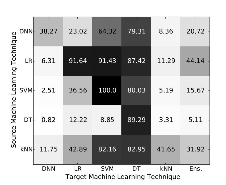
The values in each cell are the percent of samples (MNIST images here, the de facto test case for adversarial attacks) crafted to evade a particular model architecture, that when applied to another model architecture also changed their classification label. That is, the percentage of successful locally crafted adversarial samples that also fool the target model. Note that this figure does not include Random Forests or Boosted Decision Tree ensembles (the Ens column is a custom ensemble of the 5 existing techniques). The substitute model type is on the left side, and the model type being targeted is on the bottom. We can see some patterns:

• In general, the closer you match the architecture, the better the evasion is likely to be.
• Logistic Regression models (LR) make a good substitute model for other Logistic Regressions, Support Vector Machines (SVM), and Decision Trees.
• Decision Trees are the most vulnerable to attacks, with attacks from every architecture transferring well.
• The most resilient architecture is the Deep Neural Network (DNN).

From this, my theory is that if you can broadly match the target model’s architecture you have a better chance that your attacks against the substitute will transfer.

How will this hold up against our example datasets?

Attacking the Black Box

Our goal here is to recreate a local, substitute model with only having access to the model as a labeling oracle (i.e., the trained target models from the first post). Then we’ll execute the white box attacks from the second post against our substitute, hoping for sufficient attack transferability. While this is very similar to the processes in the first two posts, we have a couple of extra steps.

First, we need a new dataset to use for the model extraction. I selected 1500 random files from the PowerShellCorpus and ran each through a random set of obfuscations from Invoke-Obfuscation which gave me 3000 total samples. I then ran the feature extraction code against each script and generated the BlackBox.ast.csv file that’s now updated in ./datasets/ in the Invoke-Evasion repository.

The next step is model extraction, where we train a surrogate local model on the dataset labeled by the target model. To achieve this I used each target model to generate a respective set of labels for the new dataset. While these labels are not the exact truth, as none of our models were perfect, the labels reflect the decision boundary of the target model itself. I split the dataset into a standard train/test with an 80/20 ratio, like we did in the first post.

In the previous section I mentioned that the better you match your local model to the target model’s architecture, the higher the likelihood is that your crafted attack will fool the target. I wanted to see what “model reconnaissance” steps could help shed light on the target model’s architecture. The big question in my mind is determining if the target is linear, tree-based, a Neural Network, or some third option. Tree-based algorithms often work extremely well with pretty much any dataset, so my hypothesis is that Random Forests and Gradient Boosted Trees will match well against each target model dataset. Because of this, we ideally want to determine whether the model is likely a Neural Network or linear first, with tree-based the result of the process of elimination.

This is definitely an open question and something I don’t think has been heavily considered in academia. However I do want to reiterate again that I am not an expert here- if there is existing work in this area (or anyone has additional ideas) please let me know!

My two main ideas that I’ll detail shortly are:

1. Training multiple substitute models for each target labeled dataset, generating adversarial samples using the HopSkipJump attack from the Adversarial Robustness Toolbox. I’ll detail this more on this in a following section, but just know for now that this is a way to generate adversarial samples for any black box model.
2. Testing the heavy modification of a single important feature against the target to see if the model might be linear.

I started with fitting the following models on each target dataset, doing a basic cross-validated random search (using RandomizedSearchCV) for common hyperparameters for the shallow algorithms (i.e., everything but the Neural Network):

• Logistic Regression
• Support Vector Classifier with the radial basis function (rbf) kernel
• Gaussian Naive Bayes
• Random Forest
• Boosted Trees (XGBoost)
• One layer Neural Network with dropout (basic architecture, no hyperparameter tuning)

I then used HopSkipJump to generate adversarial samples for each model. For some reason, I wasn’t able to get the Neural Network to properly generate enough samples using HopSkipJump so I used the Fast Gradient Method (FGM) attack instead. Why choose these specific architectures as the local models? I wanted to select a range of things actually used in production, and wanted coverage of linear (Logistic Regression), tree ensembles (Random Forests/Boosted Trees), and Neural Networks.

These adversarial samples were run against each local model and the target model to get comparable accuracies. However, more importantly, I pulled out the specific samples misclassified by each local model. These samples were run against the target model, giving a the percentage of adversarial samples crafted against the local model that also fooled the target model. This is the transferability idea we talked about earlier. While how generally effective the total local adversarial samples were against the target is an interesting data point, what we really care about is how effective the local surrogate model is at crafting adversarial samples that fool the target model.

Next, I took the best performing logistic regression model, which is linear, and heavily modified a single coefficient for a sample to see if this affected the model output. The goal here was to see if the model was potentially linear for another point of reference.

Target Model1 (Logistic Regression)

Here’s the result of our evasion-transferability search process against the first model:

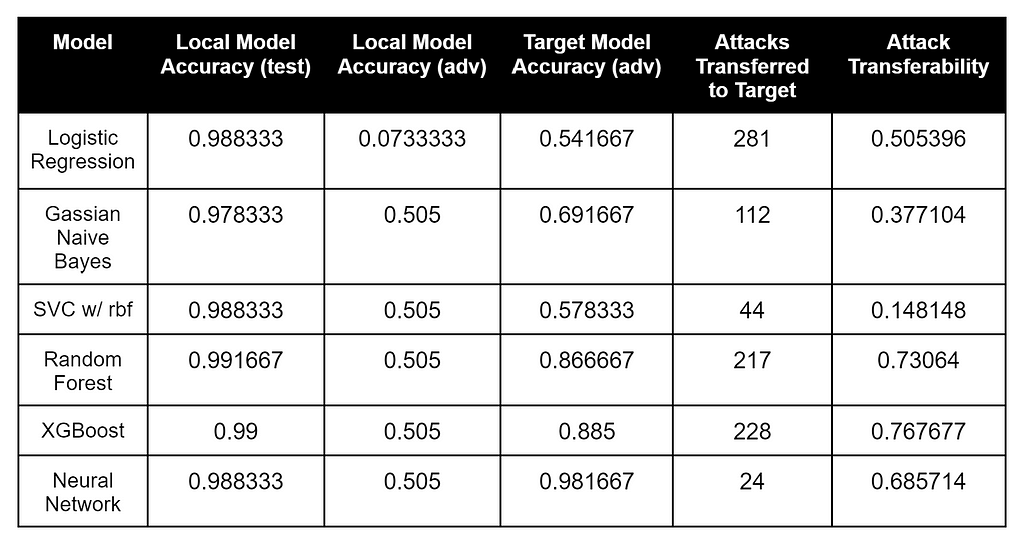
These results are interesting. The model that most closely matched the target model’s labeled data was the Random Forest, the Logistic Regression surrogate (which matched the target model’s architecture most closely) had the most number of adversarial samples transferred to the target model, but XGBoost had the highest percentage of adversarial samples that transferred to the Logistic Regression target.

Target Model2 (LightGBM)

Here’s the result of our evasion-transferability search process against the second model:

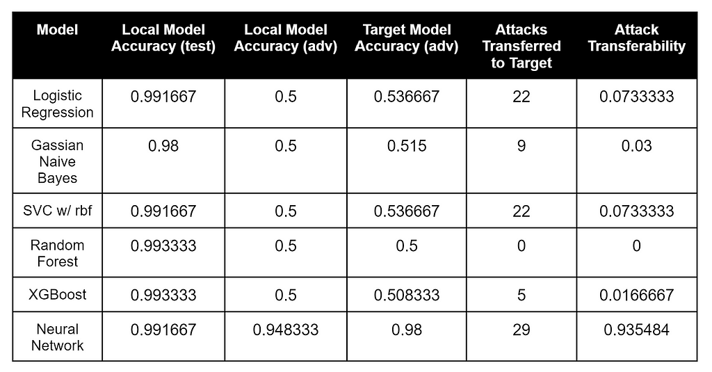
These results are also interesting. The models that most closely matched the target model’s labeled data were the Random Forest and XGBoost, while the Neural Network had both the most number of adversarial attacks that transferred as well as the best attack transferability percentage to the LightGBM target. Compared to the other two target models, Model2 appears to be the most resilient against adversarial samples as well.

Target Model3 (4 Layer Neural Network)

Here’s the result of our evasion-transferability search process against the first model:

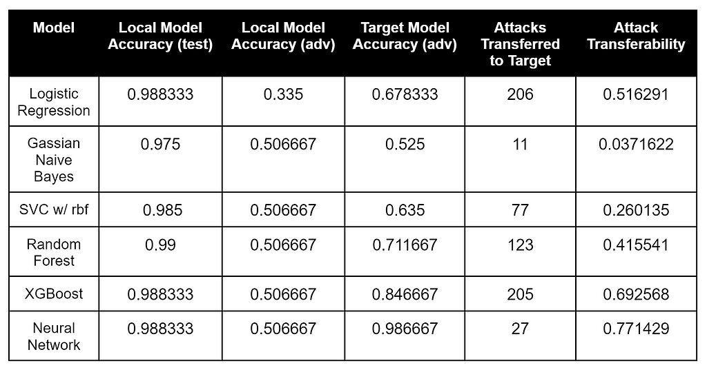
These results are just as interesting as the previous two. Most models were extremely close in accuracy on the target model’s labeled data, while the Logistic Regression and XGBoost had the most number of adversarial samples transferred to the target Neural Network. The Neural Network had the best attack transferability percentage, but the second worst number of attacks transferred.

Based on the results, my strategy to determine model architecture by measuring surrogate model attack transferability doesn’t seem like it’s working too well in this case. As a confirmation, for each model I took the most promising surrogate for each target and performed the same attacks that we did against the white box models in the second post. This didn’t end up being that effective, and I ended up with a large amount of modifications for each script. Specifically, the modified scripts would score very low in obfuscation probability against the local surrogate but would still be classified as obfuscated by the target.

I racked my brain for an explanation for this, and Will was able to help shed light on several things for me. This resulted in two major shifts in my approach: soft labels and flipping my perspective of the entire problem on its head.

Attacking the Black Box Take 2 — Soft Labels

Will details the effect of hard vs soft labels on model extraction on slide 21 from his 2021 BlackHat EU presentation:

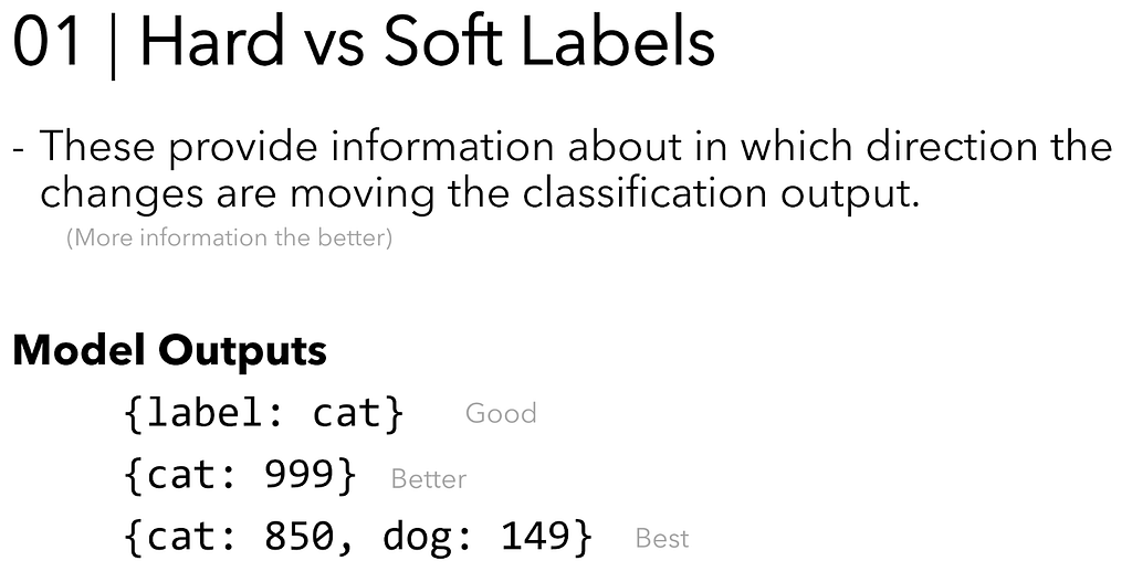
Intuitively, this makes sense. A hard label like normal or obfuscated provides less information than a set of probabilities like obfuscated=0.73. The more information we have, the better we can match the internals of the model- there’s a lot of space between hard binary labels like 0 and 1!

Let’s consider the situation where our magic Invoke-Obfuscation APIs give a probability of obfuscation like 0.73 instead of just a binary 0/1 label. How can we take advantage of this additional information? Remember back to the first post where we talked about classification versus regression: classification gives us labels, while regression gives us a number!

Let’s see what happens if we label our adversarial dataset with the probability the script is obfuscated, instead of just the hard normal/obfuscated label. We’ll keep a threshold of .5 or greater to mean the sample is obfuscated, but this can be adjusted (and often is to change the balance of false positives and false negatives).

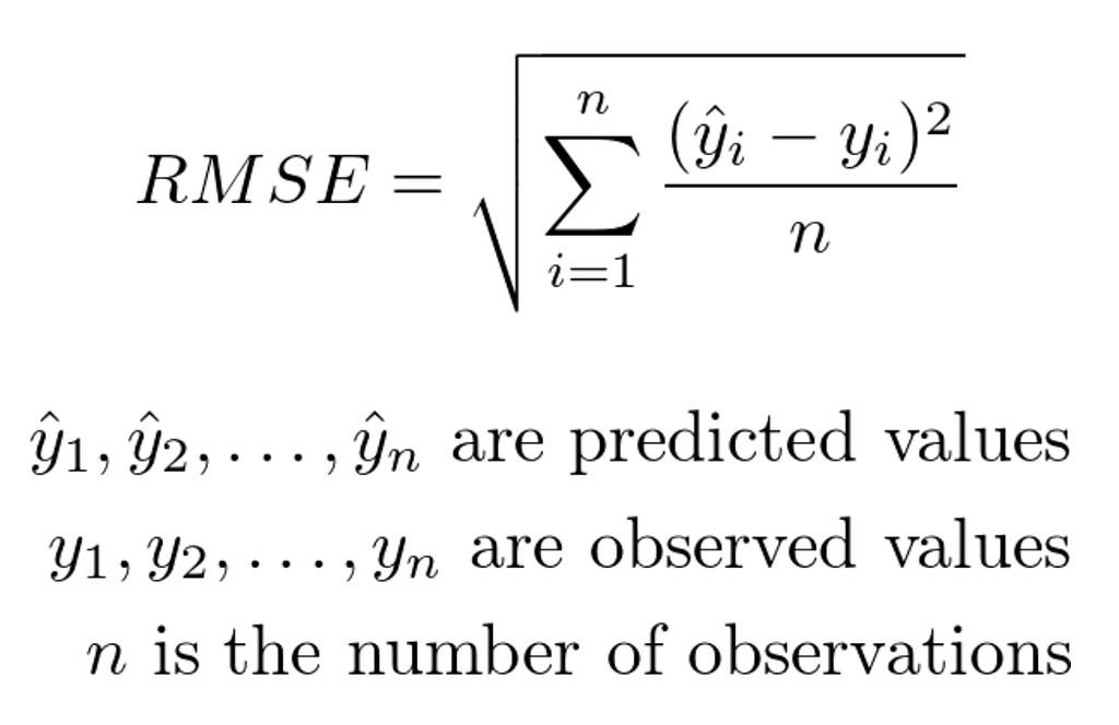
Since we’re doing regression instead of classification, we need a slightly different set of algorithms. Neural Networks, Random Forests, Gradient Boosted Trees, and Support Vector Machines all have regression equivalents. However instead of Logistic Regression (confusing name for a classifier here, I know) we’re going to use the classic Linear Regression, Lasso Regression (L1), Ridge Regression (L2), and BayesianRidge Regression instead of Bayesian Naive Bayes. Then for each, we’ll check out the Root Mean Squared Error (RMSE) on the test set, a common regression metric that squares the difference between each prediction and its actual value, adds up all of the squares, and takes the square root of the total:

We’ll also take each regression model, make a prediction for each sample, and turn those into hard labels again by seeing which are equal to .5 or above. This will let us get an accuracy measurement. This whole thing is kind of a classifier-approximating-regressors type approach. The details are in the BlackBox.ipynb notebook in the Invoke-Evasion repository.

One issue I ran into is that since we’re building regression models instead of classification models, we can’t use them out of the box with HopSkipJump or other attack algorithms. I made some attempts at rolling a custom classification model that wrapped the regression scikit-learn mode, but ART still didn’t work with them properly. I’m sure there’s a way to do this but there’s still a major issue we haven’t considered yet…

Attacking the Black Box Take 3 — The Real Problem

A big challenge I encountered while trying to wrap my head around the adversarial machine learning situation here is how to turn the modified adversarial numerical dataset back into a working script. Like I’ve mentioned over this post series, most academic adversarial machine learning research has been concerned with image data. Adversarial feature perturbation for images is pretty easy, or rather unconstrained — we just tweak the bits for pixels and then submit the image to our target classifier. Pretty much all adversarial machine learning evasion algorithms are used this way. You supply an array of data samples and an attack algorithm and perturbed/adversarial samples are produced, i.e., arrays of numbers that fool the target model when processed.

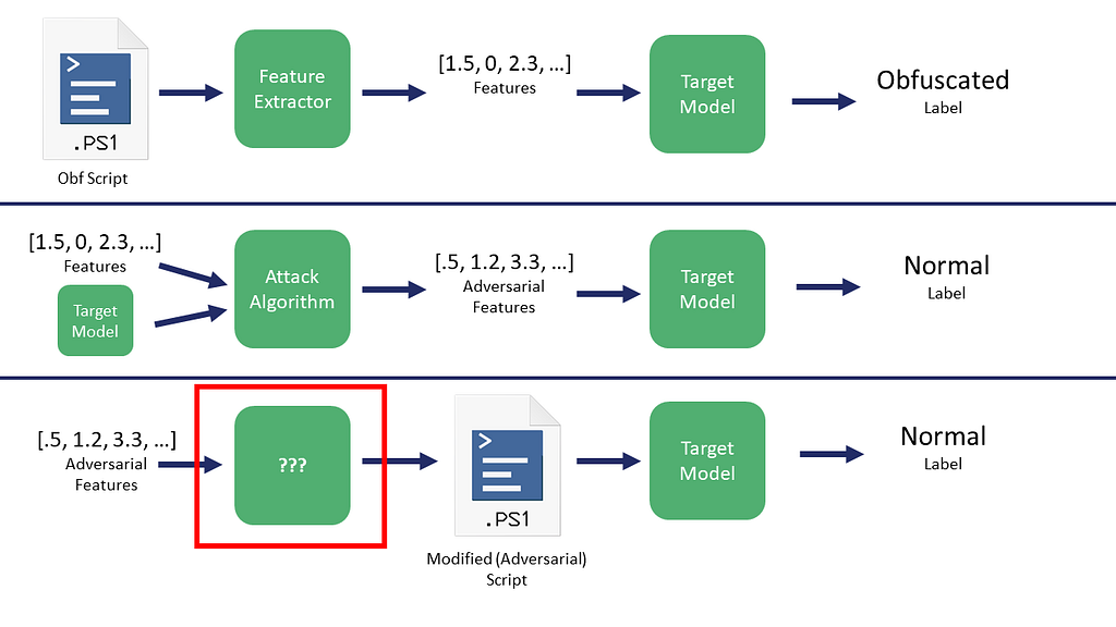
We explored the possibility of feature masking various attack algorithms in the second post on attacking white-box models. Even though we constrained the modifications to a smaller subset of more-easily-modifiable features, this still isn’t ideal. If we have an array of features modified from an original sample, how do we a) turn this back into a script that b) runs at all and c) still executes the script’s intended functionality?

Like we talked about in the second post, what is the ??? process in the following figure:

I was having difficulty wrapping my head around this until I read some of the source for the mlsecevasion branch of Counterfit and had another conversation with Will that completely changed my perspective. He relayed a key insight from Hyrum Anderson: this is all really just an optimization problem!

Black box ML attack algorithms are optimizing the measured input features for the max-min adversarial problem we talked about in the second post, where we want to maximize the error function/loss of the model for a sample but minimize the number of changes to do so. Instead of optimizing the modification of the vectorized features directly, why don’t we optimize a number of sequential actions that affect those features?

Basically, we want to first enumerate a number of modification actions we can run against a specific sample that change the features extracted for said sample. For example, Counterfit has a set of PE section adds/overlays, imports to add, and timestamps to try for PEs. For our situation, we would want something that adds “normal” features, and we can use the explainability approaches from the second post to guide this process. Then we can use an algorithm like HopSkipJump to find a combination of those features that produces the result we want.

Our approach will instead look like this:

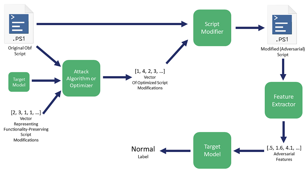
In Counterfit’s case, they’re taking a vector that represents modifications to perform and feeding this into something like HopSkipJump. For some future work I hope to build a Counterfit module for this PowerShell obfuscation, but we’ll keep things a bit more manual for now.

There’s another alternative to using attack algorithms, Bayesian Optimization, “a sequential design strategy for global optimization of black-box functions.” Remember in the first post when we briefly talked about Optuna, a framework that was built for tuning hyperparameters for machine learning algorithms. Optuna implements various Bayesian optimization methods and is super flexible, with a general approach of:

1. Define an objective function. This function has the search space for the parameter combinations you’re looking for and returns one or more objective values that need to be minimized or maximized.
2. Conduct a number of trials as part of a study, where you limit the number of trials or total running time of the study.
3. Let the math do the rest, producing an optimized set of parameters for our function!

The other key insight here is that we don’t have to use Optuna for just hyperparameter tuning! The objective function represents a black box, and we can use it to execute a number of modification actions to perform against our target script and return the obfuscation probability score from our target model. This is an approach that Counterfit implemented as well, using the Hyperopt framework instead of Optuna.

If this sounds like reinforcement learning, you’re not completely off base. Not being as literate in the relevant math as I would like, I’ll state that I believe that this approach is similar to reinforcement learning in principle but different in practice. My gut feeling is that this approach will likely work for smaller sets of atomic changes that don’t depend as much on order — larger numbers of sequential actions that are very context dependent will likely perform better with a proper reinforcement learning approach. However since we have a short feedback loop of select transforms-obfuscate script-measure obfuscation, we likely don’t need the increased overhead of a complete reinforcement learning approach.

Optimizing Obfuscation Evasion With Our Black Box

We’re going to put everything together here, combining the classifier-approximating-regressors approach with Bayesian optimization of script modifications.

Our Overall Goal: take the obfuscated DBOdemo1.ps1 input script and return a modified script that preserves the original script’s functionality while being flagged as normal by our tuned Neural Network model. We also want to add as few characters to the script as possible.

Our complete approach from start to finish will be:

1. Generate a reasonable number of obfuscated and normal samples (the positive and negative classes) and extract the vectorized features from each sample. In our case these are the 446 “most important” features selected through Borta-Shap in the first post.
2. Run the features for the vectorized samples through the target model that returns the probability of obfuscation. This produces a dataset labeled by the target “oracle” model.
3. Train a number of local regression models to fit the probability scores of the training dataset as closely as possible, measuring final performance against a hold-out test set. This step and the last constitute the Model Extraction part of the attack chain.
4. Extract feature importances from the best performing model to give us the most impactful features.
5. Examine features where the mean of the feature value is higher for normal samples than obfuscated samples. This is because we want to add normal looking code to an existing obfuscated sample.
6. Using this insight about the most normal features, manually construct multiple “script transforms” that add additional normal script data to the top of an obfuscated script. We want these transform functions to include insights from the feature importances, but also preserve the original functionality of the code. Essentially we want this code to be like script NOPs but ones that influence the model most towards the normal.
7. Build an objective function that takes an input script and applies a number of script transforms, returning the number of characters added and the obfuscation probability score from the target model instead of the local surrogate model.
8. Run an Optuna optimizer study that minimizes both of the values returned by the objective function for a multi-objective optimization.

The main insight here is that we’re extracting the target model as effectively as we can, and using the white box insights from that local surrogate model to guide the construction of functions that modify the obfuscated target script. Then we optimize the use of these modification functions against the target black box model. This approach lets us minimize the time and number of queries against the black box API.

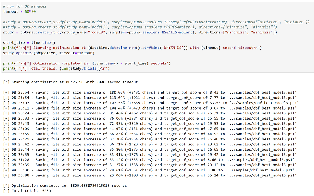
The results of our optimization study that ran for 30 minutes look like this:

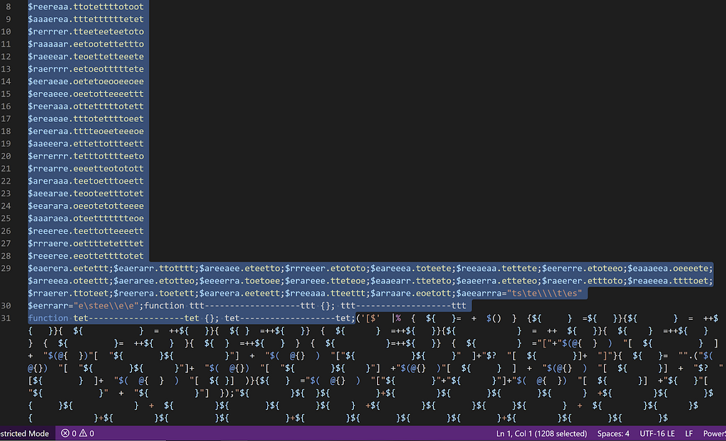
And the final optimized script looks like this:

Within 30 minutes we ended up with an optimized script that increased the original script size by only 23.06%, yet had an obfuscation score from the target model of 35.24, well below the 50 threshold for Normal.

The final question in my mind is “Does this adversarial sample transfer to the other two target models?” Let’s see:

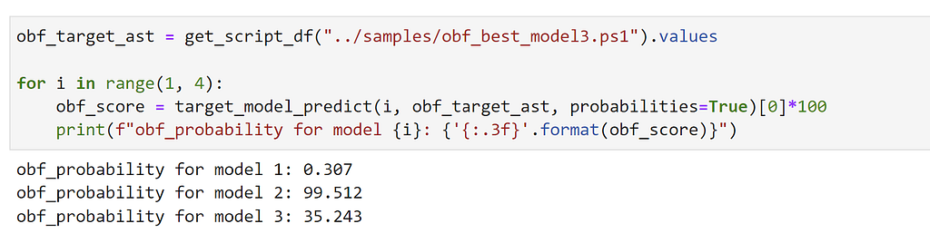
This optimized sample was successful against target model 3, the Neural Network, as well as model 1, the Logistic Regression. However it didn’t transfer to the LightGBM boosted tree-ensemble (model 2). This is likely because we:

1. Built our feature transforms from the local surrogate model tuned for model 3’s probabilities
2. Specifically optimized towards the decision boundary for model 3
3. Tree ensembles can often be more difficult to evade

Observations and Final Thoughts

Evading linear models, like Logistic Regression, is easy. Evading tree-ensembles, like Random Forests or Gradient Boosted Decision Trees, or Neural Networks, is a bit more difficult. Evading black box versions of these models is even harder, or at least takes more time and effort.

Most attacks in literature involve generating several adversarial samples and testing how effective these are against a target model, like we did for our three target models. There isn’t as much work out there that I know of (I promised I tried to look!) that involves practical real-world black box attacks tabular data like examples here. Depending on the target model architecture, and whether the model is white box or black box, evading for a single sample can have varying levels of difficulty.

The field of adversarial machine learning is less than a decade old, with the first formalized attacks being released around 2014. Most of the work thus far has been academic, and has heavily focused on white box attacks against image classifiers. While practical frameworks like the Adversarial Robustness Toolbox do exist, most of the attack algorithms have restrictions that make them either not applicable or not desirable to our security attack scenarios. Specifically, not all attack algorithms can be used on tabular/non-image data, and most do not let you limit which features are modified (known as feature masking).

From the adversarial attack algorithm side, the big insight Will relayed to me is that this is all just an optimization problem! Information security, like many industries, is often ignorant to the advances of other fields that could immensely help us. My personal example of this was when Andy and I were working on the problem/tool that eventually became the original BloodHound graph approach – we kept stumbling around the problem until Andy was discussing our challenges with his friend Sam, who lamented, “Dude, how have you guys not heard about graph theory?”

The problem of “how do we take these adversarial numbers and transform them back to a usable attack” is a real issue in executing these attacks practically. However, if we change how we think about the problem, we can use approaches influenced by the Counterfit framework, or the framework itself, to optimize adversarial actions.

My hope is that the academic adversarial machine learning community continues to make more progress on practical adversarial research beyond white box adversarial attacks on image classifiers (like this!). Real world problems are more challenging than only playing with MNIST, and there are a lot of chances for great collaboration with security industry professionals to tackle some of these practical scenarios. There are a ton of non-image-focused gradient boosted tree models deployed in the real world as black boxes: how can we go about effectively attacking them while minimizing our number of queries?

Also remember that to have pretty much any hope of an adversarial attack working against a black box model, you need to know the input features! With images, this is obvious, but for real world systems this can get more complicated and may require reverse engineering to understand feature extraction mechanisms.

And finally, remember that ML models are a “living solution”- as Lee Holmes stated, “The one thing to keep in mind with ML models or signatures is that they’re never “done”. If you’re not retraining based on false positives and false negatives, you’ve lost.” For brevity, I skipped over a lot of the real-world concerns for model deployment and maintenance. The emerging subfield of MLOps deals with a lot of these issues, and I plan to revisit the practicality of implementing the models we’ve discussed throughout this series as I learn more about this emerging discipline.

Epilogue

But what about defenses??!!?

Yes, I know I know, please don’t @ me that I’m an irresponsible red teamer. I will draft a follow-up post that reflects on some of the defenses around this problem space, however I’m still trying to get my footing for things like distillation and adversarial training. But I will leave you with an insight that adversarial ML godfather Ian Goodfellow stated around four years ago:

It’s also important to emphasize that all of the defenses so far are based on unrealistically easy threat models where the attacker is very limited…as a research problem it’s been really hard to solve even the limited version and this remains a very active research area with a lot of important challenges to solve.

For future work in this specific area, here are a few general goals I’m hoping to pursue:

• Examine text-based obfuscation detection instead of the AST approach described in this series. This affects the feasibility of deployment in some scenarios.
• Test the effectiveness of adversarial ML defenses against these specific models.
• Run this type of white/black box case study on another dataset for comparison.
• Dive more into attacking tree ensembles.
• ???

Now that we’re at the end of this firehose of information spread over three posts, I hope you enjoyed reading this material as much as I enjoyed researching and writing it. This has been a long but rewarding journey for me, and if this has sparked your interest in this field I say jump in! You can join us in the DEF CON AI Village Discord, the #DeepThought channel on the BloodHound Slack, or feel free to email me at will [at] harmj0y.net.

References

• SHAP
• The Adversarial Robustness Toolbox
• Counterfit (especially the mlsecevasion branch)
• These two posts by Adrian Kress on evading machine learning malware models, which were a great inspiration
• The “Machine learning from idea to reality: a PowerShell case study” post by Joost Jansen
• All of Will Pearce’s talks

---

Learning Machine Learning Part 3: Attacking Black Box Models was originally published in Posts By SpecterOps Team Members on Medium, where people are continuing the conversation by highlighting and responding to this story.